BMI 707 Lecture 2: Backprop, Perceptrons, and MLPs
Andrew Beam, PhD
Department of Biomedical Informatics
March 28th, 2018
twitter: @AndrewLBeam
WHAT IS A NEURAL NET?
WHAT IS A NEURAL NET?
A neural net is made up of 3 things
WHAT IS A NEURAL NET?
A neural net is made up of 3 things
The network structure
WHAT IS A NEURAL NET?
A neural net is made up of 3 things
The network structure
The loss function
-y_i*\log(p_i) - (1-y_i)*\log(1-p_i)
WHAT IS A NEURAL NET?
A neural net is made up of 3 things
The network structure
The optimizer

The loss function
-y_i*\log(p_i) - (1-y_i)*\log(1-p_i)
NEURAL NETWORK STRUCTURE

NEURAL NET STRUCTURE
A neural net is a modular way to build a classifier
X_1
X_2
Inputs
Output
Pr(y = 1 | X_1, X_2)
WHAT IS AN ARTIFICIAL NEURON?
The neuron is the basic functional unit a neural network
X_1
X_2
Inputs
Pr(y = 1 | X_1, X_2)
Output
WHAT IS AN ARTIFICIAL NEURON?
The neuron is the basic functional unit a neural network
X_1
X_2
Inputs
Pr(y = 1 | X_1, X_2)
Output
WHAT IS AN ARTIFICIAL NEURON?
The neuron is the basic functional unit a neural network
X_1
X_2
A neuron does two things, and only two things
WHAT IS AN ARTIFICIAL NEURON?
The neuron is the basic functional unit a neural network
X_2
Weight for
X_1
A neuron does two things, and only two things
Weight for
X_2
1) Weighted sum of inputs
w_1*X_1 + w_2*X_2
X_1
WHAT IS AN ARTIFICIAL NEURON?
The neuron is the basic functional unit a neural network
X_1
X_2
Weight for
X_1
A neuron does two things, and only two things
Weight for
X_2
1) Weighted sum of inputs
\phi(w_1*X_1 + w_2*X_2)
2) Nonlinear transformation
w_1*X_1 + w_2*X_2
WHAT IS AN ARTIFICIAL NEURON?

\phi()
is known as the activation function, and there are many choices
Sigmoid


Hyperbolic Tangent

WHAT IS AN ARTIFICIAL NEURON?
\phi()
is known as the activation function, and there are many choices
Sigmoid
Hyperbolic Tangent
Today
WHAT IS AN ARTIFICIAL NEURON?
\phi()
is known as the activation function, and there are many choices
Sigmoid
Hyperbolic Tangent
Today
HW 1B
WHAT IS AN ARTIFICIAL NEURON?
Summary: A neuron produces a single number that is a nonlinear transformation of its input connections
X_1
X_2
A neuron does two things, and only two things
= a number
NEURAL NETWORK STRUCTURE
X_1
X_2
Inputs
Output
Pr(y = 1 | X_1, X_2)
Neural nets are organized into layers
NEURAL NETWORK STRUCTURE
X_1
X_2
Inputs
Output
Pr(y = 1 | X_1, X_2)
Input Layer
Neural nets are organized into layers
NEURAL NETWORK STRUCTURE
X_1
X_2
Inputs
Output
Pr(y = 1 | X_1, X_2)
Neural nets are organized into layers
1st Hidden Layer
Input Layer
NEURAL NETWORK STRUCTURE
X_1
X_2
Inputs
Output
Pr(y = 1 | X_1, X_2)
Neural nets are organized into layers
A single hidden unit
1st Hidden Layer
Input Layer
NEURAL NETWORK STRUCTURE
X_1
X_2
Inputs
Output
Pr(y = 1 | X_1, X_2)
Input Layer
Neural nets are organized into layers
1st Hidden Layer
A single hidden unit
2nd Hidden Layer
NEURAL NETWORK STRUCTURE
X_1
X_2
Inputs
Output
Pr(y = 1 | X_1, X_2)
Input Layer
Neural nets are organized into layers
1st Hidden Layer
A single hidden unit
2nd Hidden Layer
Output Layer
LOSS FUNCTIONS
Output
Pr(y = 1 | X_1, X_2)
Output Layer
We need a way to measure how well the network is performing, e.g. is it making good predictions?
LOSS FUNCTIONS
Output
Pr(y = 1 | X_1, X_2)
Output Layer
We need a way to measure how well the network is performing, e.g. is it making good predictions?
Loss function: A function that returns a single number which indicates how closely a prediction matches the ground truth label
LOSS FUNCTIONS
Output
Pr(y = 1 | X_1, X_2)
Output Layer
We need a way to measure how well the network is performing, e.g. is it making good predictions?
small loss = good
big loss = bad
Loss function: A function that returns a single number which indicates how closely a prediction matches the ground true label
LOSS FUNCTIONS
A classic loss function for binary classification is binary cross-entropy
\ell(y_i,p_i) = -y_i*\log(p_i) - (1-y_i)*\log(1-p_i)
LOSS FUNCTIONS
A classic loss function for binary classification is binary cross-entropy
\ell(y_i,p_i) = -y_i*\log(p_i) - (1-y_i)*\log(1-p_i)
| y | p | Loss |
|---|---|---|
| 0 | 0.1 | 0.1 |
| 0 | 0.9 | 2.3 |
| 1 | 0.1 | 2.3 |
| 1 | 0.9 | 0.1 |
OUTPUT LAYER & LOSS
Output Layer
The output layer needs to "match" the loss function
- Correct shape
- Correct scale
\ell(y_i,p_i) = -y_i*\log(p_i) - (1-y_i)*\log(1-p_i)
OUTPUT LAYER & LOSS
Output Layer
The output layer needs to "match" the loss function
For binary cross-entropy, network needs to produce a single probability
\ell(y_i,p_i) = -y_i*\log(p_i) - (1-y_i)*\log(1-p_i)
OUTPUT LAYER & LOSS
Output Layer
The output layer needs to "match" the loss function
One unit in output layer to represent this probability
\ell(y_i,p_i) = -y_i*\log(p_i) - (1-y_i)*\log(1-p_i)
For binary cross-entropy, network needs to produce a single probability
OUTPUT LAYER & LOSS
Output Layer
The output layer needs to "match" the loss function
One unit in output layer to represent this probability
\ell(y_i,p_i) = -y_i*\log(p_i) - (1-y_i)*\log(1-p_i)
For binary cross-entropy, network needs to produce a single probability
Activation function must "squash" output to be between 0 and 1
We can change the output layer & loss to model many different kinds of data
- Multiple classes
- Continuous response (i.e. regression)
- Survival data
- Combinations of the above
THE OPTIMIZER
Question:
Now that we have specified:
- A network
- Loss function
How do we find the values for the weights that gives us the smallest possible value for the loss function?
How do we minimize the loss function?

Stochastic Gradient Decscent
- Give weights random initial values
- Evaluate partial derivative of each weight with respect negative log-likelihood at current weight value on a mini-batch
- Take a step in direction opposite to the gradient
- Rinse and repeat
THE OPTIMIZER
How do we minimize the loss function?
THE OPTIMIZER

Many variations on basic idea of SGD are available
PERCEPTRON BY HAND
PERCEPTRONS
Let's say we'd like to have a single neural learn a simple function
y
X_1
X_2
| X1 | X2 | y |
|---|---|---|
| 0 | 0 | 0 |
| 0 | 1 | 1 |
| 1 | 0 | 1 |
| 1 | 1 | 1 |
w_1
w_1
b
Observations
PERCEPTRONS
How do we make a prediction for each observations?
y
X_1
X_2
| X1 | X2 | y |
|---|---|---|
| 0 | 0 | 0 |
| 0 | 1 | 1 |
| 1 | 0 | 1 |
| 1 | 1 | 1 |
w_1
w_1
b
Assume we have the following values
| w1 | w2 | b |
|---|---|---|
| 1 | -1 | 0 |
Observations
Predictions
For the first observation:
Assume we have the following values
| w1 | w2 | b |
|---|---|---|
| 1 | -1 | 0 |
X_1 = 0, X_2 = 0, y =0
Predictions
For the first observation:
Assume we have the following values
| w1 | w2 | b |
|---|---|---|
| 1 | -1 | -0.5 |
X_1 = 0, X_2 = 0, y =0
First compute the weighted sum:
h = w_1*X_1 + w_2*X_2 + b
h = 1*0 + -1*0 + (-0.5)
h = -0.5
Predictions
For the first observation:
Assume we have the following values
| w1 | w2 | b |
|---|---|---|
| 1 | -1 | -0.5 |
X_1 = 0, X_2 = 0, y =0
First compute the weighted sum:
h = w_1*X_1 + w_2*X_2 + b
h = 1*0 + -1*0 + -0.5
h = -0.5
Transform to probability:
p = \frac{1}{1+\exp(-h)}
p = \frac{1}{1+\exp(-0.5)}
p = 0.38
Round to get prediction:
\hat{y} = round(p)
\hat{y} = 0
Predictions
Putting it all together:
h = w_1*X_1 + w_2*X_2 + b
p = \frac{1}{1+\exp(-h)}
\hat{y} = round(p)
Assume we have the following values
| w1 | w2 | b |
|---|---|---|
| 1 | -1 | -0.5 |
| X1 | X2 | y | h | p | |
|---|---|---|---|---|---|
| 0 | 0 | 0 | -0.5 | 0.38 | 0 |
| 0 | 1 | 1 | -1.5 | 0.18 | 0 |
| 1 | 0 | 1 | 0.5 | .62 | 1 |
| 1 | 1 | 1 | -0.5 | 0.38 | 0 |
\hat{y}
Fill out this table
Room for Improvement
Our neural net isn't so great... how do we make it better?
What do I even mean by better?
Room for Improvement
Let's define how we want to measure the network's performance.
There are many ways, but let's use squared-error:
(y - p)^2
Room for Improvement
Let's define how we want to measure the network's performance.
There are many ways, but let's use squared-error:
Now we need to find values for that make this error as small as possible
(y - p)^2
w_1, w_2, b
ALL OF ML IN ONE SLIDE
Our task is learning values for such the the difference between the predicted and actual values is as small as possible.
w_1, w_2, b
Learning from Data
So, how we find the "best" values for
w_1, w_2, b
Learning from Data
So, how we find the "best" values for
hint: calculus
w_1, w_2, b
Learning from Data
Recall (without PTSD) that the derivative of a function tells you how it is changing at any given location.
If the derivative is positive, it means it's going up.
If the derivative is negative, it means it's going down.
Learning from Data
Simple strategy:
- Start with initial values for
- Take partial derivatives of loss function
with respect to
- Subtract the derivative (also called the gradient) from each
w_1, w_2, b
w_1, w_2, b
The Backpropagation Algorithm


The Backpropagation Algorithm
h = w_1*X_1 + w_2*X_2 + b
p = \frac{1}{1+\exp(-h)}
Our perception performs the following computations
\ell = (y - p)^2
And we want to minimize this quantity
The Backpropagation Algorithm
h = w_1*X_1 + w_2*X_2 + b
p = \frac{1}{1+\exp(-h)}
Our perception performs the following computations
\ell = (y - p)^2
And we want to minimize this quantity
We'll compute the gradients for each parameter by "back-propagating" errors through each component of the network
The Backpropagation Algorithm
For we need to compute
h = w_1*X_1 + w_2*X_2 + b
Computations
p = \frac{1}{1+\exp(-h)}
Loss
w_1
\frac{\partial \ell}{\partial w_1}
\ell = (y - p)^2
To get there, we will use the chain rule
\frac{\partial \ell}{\partial w_1} = \frac{\partial \ell}{\partial p}*\frac{\partial p}{\partial h}*\frac{\partial h}{\partial w_1}
This is "backprop"
The Backpropagation Algorithm
Let's break it into pieces
h = w_1*X_1 + w_2*X_2 + b
Computations
p = \frac{1}{1+\exp(-h)}
Loss
\ell = (y - p)^2
\frac{\partial \ell}{\partial w_1} = \frac{\partial \ell}{\partial p}*\frac{\partial p}{\partial h}*\frac{\partial h}{\partial w_1}
\frac{\partial \ell}{\partial p} = ?
The Backpropagation Algorithm
Let's break it into pieces
h = w_1*X_1 + w_2*X_2 + b
Computations
p = \frac{1}{1+\exp(-h)}
Loss
\ell = (y - p)^2
\frac{\partial \ell}{\partial w_1} = \frac{\partial \ell}{\partial p}*\frac{\partial p}{\partial h}*\frac{\partial h}{\partial w_1}
\frac{\partial \ell}{\partial p} = 2*(p-y)
\frac{\partial p}{\partial h} = ?
The Backpropagation Algorithm
Let's break it into pieces
h = w_1*X_1 + w_2*X_2 + b
Computations
p = \frac{1}{1+\exp(-h)}
Loss
\ell = (y - p)^2
\frac{\partial \ell}{\partial w_1} = \frac{\partial \ell}{\partial p}*\frac{\partial p}{\partial h}*\frac{\partial h}{\partial w_1}
\frac{\partial \ell}{\partial p} = 2*(p-y)
\frac{\partial p}{\partial h} = p*(1-p)
\frac{\partial h}{\partial w} = ?
The Backpropagation Algorithm
Let's break it into pieces
h = w_1*X_1 + w_2*X_2 + b
Computations
p = \frac{1}{1+\exp(-h)}
Loss
\ell = (y - p)^2
\frac{\partial \ell}{\partial w_1} = \frac{\partial \ell}{\partial p}*\frac{\partial p}{\partial h}*\frac{\partial h}{\partial w_1}
\frac{\partial \ell}{\partial p} = 2*(p-y)
\frac{\partial p}{\partial h} = p*(1-p)
\frac{\partial h}{\partial w_1} = X_1
\frac{\partial \ell}{\partial w_1} = 2*(p-y)*p*(1-p)*X_1
Putting it all together
Gradient Descent with Backprop
gw_1 = \eta*(p - y)*(p*(1-p)*X_1)
1) Compute the gradient for
w^{new}_1 = w^{old}_1 - \sum gw_1
2) Update
w_1
w_1
\eta
is the learning rate
For some number of iterations we will:
3) Repeat until "convergence"
Learning Rules for each Parameter
gw_1 = (p - y)*(p*(1-p)*X_1)
gw_2 = (p - y)*(p*(1-p)*X_2)
g_b = (p - y)*(p*(1-p))
Gradient for
Gradient for
Gradient for
w^{new}_1 = w^{old}_1 - \eta*\frac{1}{N}\sum gw_1
Update for
Update for
Update for
w^{new}_2 = w^{old}_2 - \eta*\frac{1}{N}\sum gw_2
b^{new} = b^{old} - \eta*\frac{1}{N}\sum g_b
w_1
w_1
w_2
w_2
b
b
\eta
is the learning rate
Learning Rules for each Parameter
\eta
is the learning rate
Fill in new table!
w^{new}_1 = w^{old}_1 - \eta*\frac{1}{N}\sum gw_1
Update for
Update for
Update for
w^{new}_2 = w^{old}_2 - \eta*\frac{1}{N}\sum gw_2
b^{new} = b^{old} - \eta*\frac{1}{N}\sum g_b
w_1
w_2
b
gw_1 = (p - y)*(p*(1-p)*X_1)
gw_2 = (p - y)*(p*(1-p)*X_2)
g_b = (p - y)*(p*(1-p))
Gradient for
Gradient for
Gradient for
w_1
w_2
b
\eta
IMPLEMENTATION IN PYTHON
Another Example
| X1 | X2 | y |
|---|---|---|
| 0 | 0 | 0 |
| 0 | 1 | 0 |
| 1 | 0 | 0 |
| 1 | 1 | 1 |
Final Example
| X1 | X2 | y |
|---|---|---|
| 0 | 0 | 0 |
| 0 | 1 | 1 |
| 1 | 0 | 1 |
| 1 | 1 | 0 |
What Happened?
Why didn't this work?
What Happened?
Why didn't this work?
Is this relationship "harder" in some sense?
What Happened?
Why didn't this work?
Is this relationship "harder" in some sense?
Let's plot it and see.
MULTILAYER PERCEPTRONS
Perceptron -> MLP
With a small change, we can turn our perceptron model into a multilayer perceptron
- Instead of just one linear combination, we are going to take several, each with a different set of weights (called a hidden unit)
- Each linear combination will be followed by a nonlinear activation
- Each of these nonlinear features will be fed into the logistic regression classifier
- All of the weights are learned end-to-end via SGD
MLPs learn a set of nonlinear features directly from data
"Feature learning" is the hallmark of deep learning approachs
MULTILAYER PERCEPTRONS (MLPs)
Let's set up the following MLP with 1 hidden layer that has 3 hidden units:
X_1
X_2
Pr(y = 1 | X_1, X_2)
Each neuron in the hidden layer is going to do exactly the same thing as before.
h_1
h_2
h_3
o
MULTILAYER PERCEPTRONS (MLPs)
X_1
X_2
h_1
h_2
h_3
o
Computations are:
o = b_o + \sum^3_{j=1} w_{oj}*h_j
p
p = \frac{1}{1 + exp(-o)}
h_j = \phi(w_{1j}*X_1 + w_{2j}*X_2 + b_j)
MULTILAYER PERCEPTRONS (MLPs)
X_1
X_2
h_1
h_2
h_3
o
Computations are:
o = b_o + \sum^3_{j=1} w_{oj}*h_j
p
p = \frac{1}{1 + exp(-o)}
h_j = \phi(w_{1j}*X_1 + w_{2j}*X_2 + b_j)
Output layer weight derivatives
\frac{\partial \ell}{\partial w_{oj}} = \frac{\partial \ell}{\partial p}*\frac{\partial p}{\partial o}*\frac{\partial o}{\partial w_{oj}}
= (p-y)*p*(1-p)*h_j
MULTILAYER PERCEPTRONS (MLPs)
X_1
X_2
h_1
h_2
h_3
o
Computations are:
o = b_o + \sum^3_{j=1} w_{oj}*h_j
p
p = \frac{1}{1 + exp(-o)}
h_j = \phi(w_{1j}*X_1 + w_{2j}*X_2 + b_j)
\frac{\partial \ell}{\partial w_{1j}} = \frac{\partial \ell}{\partial p}*\frac{\partial p}{\partial o}*\frac{\partial o}{\partial h}*\frac{\partial h}{\partial w_{1j}}
Hidden layer weight derivatives
\frac{\partial \ell}{\partial w_{oj}} = \frac{\partial \ell}{\partial p}*\frac{\partial p}{\partial o}*\frac{\partial o}{\partial w_{oj}}
Output layer weight derivatives
= (p-y)*p*(1-p)*h_j
= (p-y)*p*(1-p)*h_j*(1-h_j)*X_1
(if we use a sigmoid activation function)
MLP Terminology
X_1
X_2
Pr(y = 1 | X_1, X_2)
h_1
h_2
h_3
o
X_1
X_2
Pr(y = 1 | X_1, X_2)
h_1
h_2
h_3
o
Forward pass = computing probability from input
MLP Terminology
X_1
X_2
Pr(y = 1 | X_1, X_2)
h_1
h_2
h_3
o
Forward pass = computing probability from input
MLP Terminology
Backward pass = computing derivatives from output
X_1
X_2
Pr(y = 1 | X_1, X_2)
h_1
h_2
h_3
o
Forward pass = computing probability from input
MLP Terminology
Backward pass = computing derivatives from output
Hidden layers are often called "dense" layers
MULTILAYER PERCEPTRONS (MLPs)
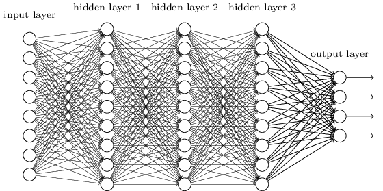
We can increase the flexibility by adding more layers
MULTILAYER PERCEPTRONS (MLPs)
We can increase the flexibility by adding more layers
but we run the risk of overfitting...
REGULARIZATION
REGULARIZATION
One of the biggest problems with neural networks is overfitting.
Regularization schemes combat overfitting in a variety of different ways
REGULARIZATION
A perceptron represents the following optimization problem:
\text{argmin}_{W} \ \ell(y, f(X))
where
f(X) = \frac{1}{1+exp(-\phi(XW))}
REGULARIZATION
One way to regularize is introduce penalties and change
\text{argmin}_{W} \ \ell(y, f(X))
REGULARIZATION
\text{argmin}_{W} \ \ell(y, f(X))
to
\text{argmin}_{W} \ \ell(y, f(X)) + \lambda R(W)
One way to regularize is introduce penalties and change
REGULARIZATION
A familiar why to regularize is introduce penalties and change
\text{argmin}_{W} \ \ell(y, f(X))
to
\text{argmin}_{W} \ \ell(y, f(X)) + \lambda R(W)
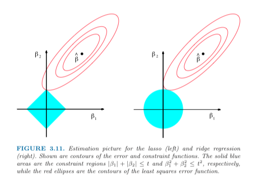
where R(W) is often the L1 or L2 norm of W. These are the well known ridge and LASSO penalties, referred to as weight decay by neural net community
L2 REGULARIZATION
We can limit the size of the L2 norm of the weight vector:
\text{argmin}_{W} \ \ell(y, f(X)) + \lambda ||W||_2
where
||W||_2 = \sum^p_{j=1} w_j^2
L1/L2 REGULARIZATION
We can limit the size of the L2 norm of the weight vector:
\text{argmin}_{W} \ \ell(y, f(X)) + \lambda ||W||_2
where
||W||_2 = \sum^p_{j=1} w_j^2
We can do the same for the L1 norm. What do these penalties do?
SHRINKAGE
L1 and L2 penalties shrink the weights towards 0
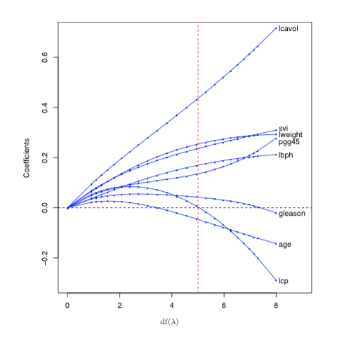
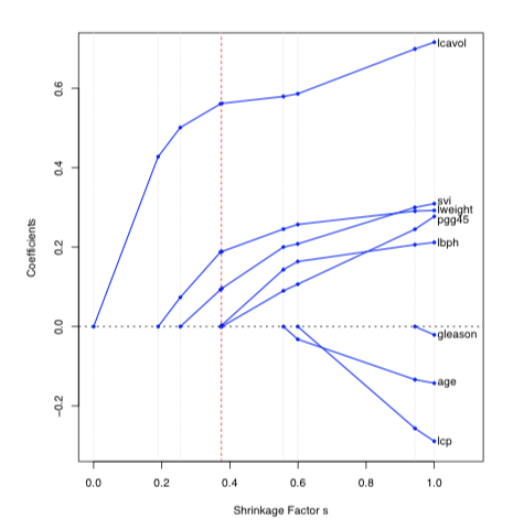
L2 Penalty
L1 Penalty
Friedman, Jerome, Trevor Hastie, and Robert Tibshirani. The elements of statistical learning. Vol. 1. New York: Springer series in statistics, 2001.
SHRINKAGE
L1 and L2 penalties shrink the weights towards 0
Friedman, Jerome, Trevor Hastie, and Robert Tibshirani. The elements of statistical learning. Vol. 1. New York: Springer series in statistics, 2001.
SHRINKAGE
L1 and L2 penalties shrink the weights towards 0
Friedman, Jerome, Trevor Hastie, and Robert Tibshirani. The elements of statistical learning. Vol. 1. New York: Springer series in statistics, 2001.
Why is this a "good" idea?
STOCHASTIC REGULARIZATION
Often, we will inject noise into the neural network during training. By far the most popular way to do this is dropout
STOCHASTIC REGULARIZATION
Often, we will inject noise into the neural network during training. By far the most popular way to do this is dropout
Given a hidden layer, we are going to set each element of the hidden layer to 0 with probability p each SGD update.

STOCHASTIC REGULARIZATION
One way to think of this is the network is trained by bagged versions of the network. Bagging reduces variance.
STOCHASTIC REGULARIZATION
One way to think of this is the network is trained by bagged versions of the network. Bagging reduces variance.
Others have argued this is an approximate Bayesian model
STOCHASTIC REGULARIZATION
Many have argued that SGD itself provides regularization
INITIALIZATION REGULARIZATION
The weights in a neural network are given random values initially
INITIALIZATION REGULARIZATION
The weights in a neural network are given random values initially
There is an entire literature on the best way to do this initialization
INITIALIZATION REGULARIZATION
The weights in a neural network are given random values initially
There is an entire literature on the best way to do this initialization
- Normal
- Truncated Normal
- Uniform
- Orthogonal
- Scaled by number of connections
- etc
INITIALIZATION REGULARIZATION
Try to "bias" the model into initial configurations that are easier to train
INITIALIZATION REGULARIZATION
Try to "bias" the model into initial configurations that are easier to train
Very popular way is to do transfer learning
INITIALIZATION REGULARIZATION
Try to "bias" the model into initial configurations that are easier to train
Very popular way is to do transfer learning
Train model on auxiliary task where lots of data is available
INITIALIZATION REGULARIZATION
Try to "bias" the model into initial configurations that are easier to train
Very popular way is to do transfer learning
Train model on auxiliary task where lots of data is available
Use final weight values from previous task as initial values and "fine tune" on primary task
STRUCTURAL REGULARIZATION
However, the key advantage of neural nets is the ability to easily include properties of the data directly into the model through the network's structure
Convolutional neural networks (CNNs) are a prime example of this (Kun will discuss CNNs)
Conclusions
Backprop, perceptrons, and MLPS are the "building" blocks of neural nets
You'll get a chance to demonstrate your mastery in HW 1A and 1B.
We will reuse these concepts for the rest of the semester.
Conclusions

BMI 707 - Lecture 2: Backprop, Perceptrons, and MLPs
By beamandrew
