DEEP LEARNING 101

Andrew Beam, PhD

Postdoctoral Fellow

Department of Biomedical Informatics

Harvard Medical School

February 24th, 2017

twitter: @AndrewLBeam

GOAL OF THIS TALK

THIS TALK IS A MULTIMEDIA EXPERIENCE

Deep Learning 101 companion series of blog posts:

http://beamandrew.github.io

Jupyter Notebooks:

https://github.com/beamandrew/deeplearning_101

DEEP LEARNING HAS MASTERED GO

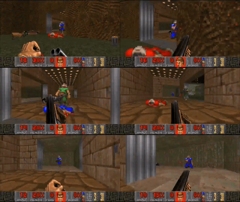
DEEP LEARNING CAN PLAY VIDEO GAMES

DEEP LEARNING CAN IMITATE STYLE

EVERYONE IS USING DEEP LEARNING

WHAT IS A NEURAL NET?

NEURAL NETWORKS ARE AN OLD IDEA

One of the very first ideas in machine learning and artificial intelligence

Date back to 1940s
Many cycles of boom and bust
Repeated promises of "true AI" that were unfulfilled followed by "AI winters"

Are today's neural nets any different than their predecessors?

"[The perceptron is] the embryo of an electronic computer that [the Navy] expects will be able to walk, talk, see, write, reproduce itself and be conscious of its existence." - Frank Rosenblatt, 1958

MILESTONES

IN THE BEGINNING... (1940s-1960s)

Warren McCulloch and Walter Pitts (1943)

Thresholded logic unit with hardcoded weights

Intended to mimic "integrate and fire" model of neurons

IN THE BEGINNING... (1940s-1960s)

Rosenblatt's Perceptron, 1957

Initially very promising
Came with provably correct learning algorithm
Could recognize letters and numbers

THE FIRST AI WINTER (1969)

Minsky and Papert show that the perceptron can't even solve the XOR problem

Kills research on neural nets for the next 15-20 years

THE BACKPROPAGANDISTS EMERGE (1986)

Rumelhart, Hinton, and Willams show us how to train multilayered neural networks

REBRANDING AS 'DEEP LEARNING' (2006)

Unsupervised pre-training of "deep belief nets" allowed for large and deeper models

Image credit: https://www.toptal.com/machine-learning/an-introduction-to-deep-learning-from-perceptrons-to-deep-networks

THE BREAKTHROUGH (2012)

Imagenet Database

Millions of labeled images
Objects in images fall into 1 of a possible 1,000 categories
Relatively high-resolution
Bounding boxes giving exact location of object - useful for both classification and localization

Large Scale Visual

Recognition Challenge (ILSVRC)

Annual Imagenet Challenge starting in 2010
Successor to smaller PASCAL VOC challenge
Many tracks including classification and localization
Standardized training and test set. Competitors upload predictions for test set and are automatically scored

THE BREAKTHROUGH (2012)

Pivotal event occurred in an image recognition contest which brought together 3 critical ingredients for the first time:

Massive amounts of labeled images
Training with GPUs
Methodological innovations that enabled training deeper networks while minimizing overfitting

THE BREAKTHROUGH (2012)

In 2011, a misclassification rate of 25% was near state of the art on ILSVRC

In 2012, Geoff Hinton and two graduate students, Alex Krizhevsky and Ilya Sutskever, entered ILSVRC with one of the first deep neural networks trained on GPUs, now known as "Alexnet"

Result: An error rate of 16%, nearly half what the second place entry was able to achieve.

The computer vision world immediately took notice

THE ILSVRC AFTERMATH (2012-2014)

Alexnet paper has ~ 10,000 citations since being published in 2012!

NETS KEEP GETTING DEEPER (2012-2016)

WHAT'S CHANGED? WHY NOW?

Several key advancements has enabled the modern deep learning revolution

WHAT'S CHANGED? WHY NOW?

Several key advancements have enabled the modern deep learning revolution

Availability of massive datasets

with high-quality labels

Standardized benchmarks of progress and open source tools

Community acknowledgment that

open data -> everyone gets better

WHAT'S CHANGED? WHY NOW?

Several key advancements have enabled the modern deep learning revolution

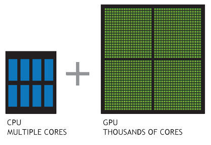
Advent of massively parallel computing by GPUs. Enabled training of huge neural nets on extremely large datasets

WHAT'S CHANGED? WHY NOW?

Several key advancements have enabled the modern deep learning revolution

Methodological advancements have made deeper networks easier to train

Architecture

Optimizers

Activation Functions

WHAT'S CHANGED? WHY NOW?

Several key advancements have enabled the modern deep learning revolution

Robust frameworks and abstractions make iteration faster and less error prone

Automatic differentiation allows easy prototyping

WHAT'S CHANGED? WHY NOW?

This all leads to the following hypothesis

Deep Learning Hypothesis: The success of deep learning is largely a success of engineering.

Personal belief: Things are different with neural nets this time around

WHAT'S CHANGED? WHY NOW?

Fitting Analogy?

WHAT'S CHANGED? WHY NOW?

These advancements have been transferred to other fields

Doctors were crucial... in creating the labeled dataset!

WHAT'S CHANGED? WHY NOW?

These advancements have been transferred to other fields

Off the shelf, pre-trained deep neural network + 130,000 images = expert level diagnostic accuracy

WHAT'S CHANGED? WHY NOW?

Not just medicine, but genomics too

More here: https://github.com/gokceneraslan/awesome-deepbio

HOW CAN YOU STAY CURRENT?

The field moves fast, staying up to date can be challenging

http://beamandrew.github.io/deeplearning/2017/02/23/deep_learning_101_part1.html

DEEP LEARNING AND YOU

Barrier to entry for deep learning is actually low

... but a few things might stand in your way:

Need to make sure your problem is a good fit
- Lots of labeled data and appropriate signal/noise ratio
Access to GPUs
Must "speak the language"
- Many design choices and hyper parameter selections
Know how to "babysit" the model during learning phase

Introduction to Deep Learning Models

MULTILAYER PERCEPTRONS (MLPs)

Most generic form of a neural net is the "multilayer perceptron"
Input undergoes a series of nonlinear transformation before a final classification layer

MULTILAYER PERCEPTRONS (MLPs)

MLPs are the easiest entry point to understand what's going on in a deep learning model
Closely related to logistic regression

LOGISTIC REGRESSION REFRESHER

Pretend we just have two variables:

x_1,x_2

x_1,x_2

... and a class label:

y \in \{0,1\}

y \in \{0,1\}

LOGISTIC REGRESSION REFRESHER

f(x_1,x_2) := w_0 + x_{i1} * w_1 + x_{i2} * w_2

f(x_1,x_2) := w_0 + x_{i1} * w_1 + x_{i2} * w_2

Pretend we just have two variables:

x_1,x_2

x_1,x_2

... and a class label:

y \in \{0,1\}

y \in \{0,1\}

... we construct a function to predict y from x:

LOGISTIC REGRESSION REFRESHER

f(x_1,x_2) := w_0 + x_{i1} * w_1 + x_{i2} * w_2

f(x_1,x_2) := w_0 + x_{i1} * w_1 + x_{i2} * w_2

Pretend we just have two variables:

x_1,x_2

x_1,x_2

... and a class label:

y \in \{0,1\}

y \in \{0,1\}

... we construct a function to predict y from x:

p(x_1,x_2) := \frac{1}{1+\exp(-f(x_1,x_2))}

p(x_1,x_2) := \frac{1}{1+\exp(-f(x_1,x_2))}

... and turn this into a probability using the logistic function:

LOGISTIC REGRESSION REFRESHER

f(x_1,x_2) := w_0 + x_{i1} * w_1 + x_{i2} * w_2

f(x_1,x_2) := w_0 + x_{i1} * w_1 + x_{i2} * w_2

Pretend we just have two variables:

x_1,x_2

x_1,x_2

... and a class label:

y \in \{0,1\}

y \in \{0,1\}

... we construct a function to predict y from x:

p(x_1,x_2) := \frac{1}{1+\exp(-f(x_1,x_2))}

p(x_1,x_2) := \frac{1}{1+\exp(-f(x_1,x_2))}

... and turn this into a probability using the logistic function:

\ell(w|x) := -y*\log(p(x)) - (1-y)*\log(1-p(x))

\ell(w|x) := -y*\log(p(x)) - (1-y)*\log(1-p(x))

... and use Bernoulli negative log-likelihood as loss:

LOGISTIC REGRESSION REFRESHER

f(x_1,x_2) := w_0 + x_{i1} * w_1 + x_{i2} * w_2

f(x_1,x_2) := w_0 + x_{i1} * w_1 + x_{i2} * w_2

Pretend we just have two variables:

x_1,x_2

x_1,x_2

... and a class label:

y \in \{0,1\}

y \in \{0,1\}

... we construct a function to predict y from x:

p(x_1,x_2) := \frac{1}{1+\exp(-f(x_1,x_2))}

p(x_1,x_2) := \frac{1}{1+\exp(-f(x_1,x_2))}

... and turn this into a probability using the logistic function:

This is good old-fashioned logistic regression

\ell(w|x) := -y*\log(p(x)) - (1-y)*\log(1-p(x))

\ell(w|x) := -y*\log(p(x)) - (1-y)*\log(1-p(x))

... and use Bernoulli negative log-likelihood as loss:

LOGISTIC REGRESSION REFRESHER

How do we learn the "best" values for ?

\{w_0,w_1,w_2\}

\{w_0,w_1,w_2\}

LOGISTIC REGRESSION REFRESHER

How do we learn the "best" values for ?

\{w_0,w_1,w_2\}

\{w_0,w_1,w_2\}

Gradient Decscent

Give weights random initial values
Evaluate partial derivative of each weight with respect negative log-likelihood at current weight value
Take a step in direction opposite to the gradient
Rinse and repeat

LOGISTIC REGRESSION REFRESHER

How do we learn the "best" values for ?

\{w_0,w_1,w_2\}

\{w_0,w_1,w_2\}

This in essence is the entire "learning" algorithm

behind modern deep learning. Keep this in mind.

Gradient Decscent

Give weights random initial values
Evaluate partial derivative of each weight with respect negative log-likelihood at current weight value
Take a step in direction opposite to the gradient
Rinse and repeat

LOGISTIC REGRESSION -> MLP

With a small change, we can turn our logistic regression model into a neural net

Instead of just one linear combination, we are going to take several, each with a different set of weights (called a hidden unit)
Each linear combination will be followed by a nonlinear activation
Each of these nonlinear features will be fed into the logistic regression classifier
All of the weights are learned end-to-end via SGD

MLPs learn a set of nonlinear features directly from data

"Feature learning" is the hallmark of deep learning approachs

MLPs

Can add more layers to increase capacity of network

MLP IN 8 LINES

from keras.layers import Input, Dense, Dropout
from keras.models import Sequential

mlp = Sequential()
mlp.add(Dense(output_dim=128, input_dim=num_variables, activation='relu'))
mlp.add(Dropout(0.5))
mlp.add(Dense(output_dim=1, activation='sigmoid'))
mlp.compile(optimizer='adam', loss='binary_crossentropy',metrics=['accuracy'])
mlp.fit(X_train, y_train,validation_data=[X_val,y_val],nb_epoch=10,verbose=1)

See this notebook for more details: https://github.com/beamandrew/deeplearning_101/blob/master/mlp_tutorial.ipynb

Tensorflow backend gives gradients, training procedure, GPU computation "for free"!

CONVOLUTIONAL NEURAL NETS (CNNs)

CNNs are the workhorse model in image recognition

Simplified version of MLP
"Local" weight connections
Responsible for most of the initial deep learning breakthroughs
Tailored specifically for characteristics of image recognition

CONVOLUTIONAL NEURAL NETS (CNNs)

Dates back to the late 1980s

Invented by in 1989 Yann Lecun at Bell Labs - "Lenet"
Integrated into handwriting recognition systems
in the 90s
Huge flurry of activity after the Alexnet paper

CONVOLUTIONAL NEURAL NETS

Images are just 2D arrays of numbers

Goal is to build f(image) = 1

CONVOLUTIONAL NEURAL NETS

CNNs exploit strong prior information about images

If we just "flatten" the image into a vector, we throw away a ton of information

CNNs use the structural properties of images to improve performance.

CONVOLUTIONAL NEURAL NETS

CNNs exploit strong prior information about images

What's a convolution?

In images, it just means that we're doing a dot-product over a small image patch

CONVOLUTIONAL NEURAL NETS

Example convolution

CONVOLUTIONAL NEURAL NETS

CNNs look at small connected groups of pixels using "filters"

Image credit: http://deeplearning.stanford.edu/wiki/index.php/Feature_extraction_using_convolution

Images have a local correlation structure

Near by pixels are likely to be more similar than pixels that are far away

CNNs exploit this through convolutions of small image patches

CONVOLUTIONAL NEURAL NETS

Pooling provides spatial invariance

Image credit: http://cs231n.github.io/convolutional-networks/

CONVOLUTIONAL NEURAL NETS

Convolution + pooling + activation = CNN

Image credit: http://cs231n.github.io/convolutional-networks/

CONVOLUTIONAL NEURAL NETS (CNNs)

CNN formula is relatively simple

Image credit: http://cs231n.github.io/convolutional-networks/

CONVOLUTIONAL NEURAL NETS

Data augmentation mimics the image generative process

Image credit: http://slideplayer.com/slide/8370683/

Drastically "expands" training set size
Improves generalization
Works if it doesn't "break" image -> label relationship

CNN 12 LINES OF CODE

cnn = Sequential()
cnn.add(Convolution2D(nb_filter=32,nb_row=5,nb_col=5,activation='relu'))
cnn.add(Convolution2D(nb_filter=32,nb_row=5,nb_col=5,activation='relu'))
cnn.add(MaxPooling2D(pool_size=(2, 2)))
cnn.add(Convolution2D(nb_filter=32,nb_row=5,nb_col=5,activation='relu'))
cnn.add(Convolution2D(nb_filter=32,nb_row=5,nb_col=5,activation='relu'))
cnn.add(MaxPooling2D(pool_size=(2, 2)))
cnn.add(Flatten())
cnn.add(Dense(output_dim=1024,activation='relu'))
cnn.add(Dense(output_dim=10,activation='softmax'))
cnn.compile(loss='categorical_crossentropy',optimizer='adam')
cnn.fit(X_train,Y_train,batch_size=64)

Again, tensorflow backend gives gradients, training procedure, GPU computation "for free"!

See this notebook (soon to be published) for more details: https://github.com/beamandrew/deeplearning_101/blob/master/cnn_tutorial.ipynb

ADVERSARIAL EXAMPLES

CNNs can be tricked in strange ways

Image credit: https://openai.com/blog/adversarial-example-research/

ADVERSARIAL EXAMPLES

Works on "real" photos too

Image credit: https://openai.com/blog/adversarial-example-research/

CNNS AREN'T MAGIC

Based on solid image priors
Learns a hierarchical set of filters
Exploit properties of images, e.g. local correlations and invariances
Mimic generative distribution with augmentation to reduce over fitting
Results in end-to-end visual recognition system trained with SGD on GPUs: pixels in -> classifications out

CNNs exploit strong prior information about images

HOW TO GET STARTED

https://wiki.med.harvard.edu/Orchestra/OrchestraNvidiaGPUs

HMS has GPU resources

tensorflow: module load dev/tensorflow/0.12-GPU

CONCLUSIONS

Deep learning is real and probably here to stay
Could potentially impact many fields -> understand concepts so you have deep learning "insurance"
Long history and connections to other models and fields
Prereqs: Data (lots) + GPUs (more = better)
Deep learning models are like legos, but you need to know what blocks you have and how they fit together
Need to have a sense of sensible default parameter values to get started
"Babysitting" the learning process is a skill

DEEP LEARNING 101

GOAL OF THIS TALK

THIS TALK IS A MULTIMEDIA EXPERIENCE

DEEP LEARNING HAS MASTERED GO

DEEP LEARNING CAN PLAY VIDEO GAMES

DEEP LEARNING CAN PLAY VIDEO GAMES

DEEP LEARNING CAN PLAY VIDEO GAMES

DEEP LEARNING CAN PLAY VIDEO GAMES

DEEP LEARNING CAN IMITATE STYLE

EVERYONE IS USING DEEP LEARNING

WHAT IS A NEURAL NET?

NEURAL NETWORKS ARE AN OLD IDEA

MILESTONES

IN THE BEGINNING... (1940s-1960s)

IN THE BEGINNING... (1940s-1960s)

THE FIRST AI WINTER (1969)

THE BACKPROPAGANDISTS EMERGE (1986)

REBRANDING AS 'DEEP LEARNING' (2006)

THE BREAKTHROUGH (2012)

THE BREAKTHROUGH (2012)

THE BREAKTHROUGH (2012)

THE ILSVRC AFTERMATH (2012-2014)

NETS KEEP GETTING DEEPER (2012-2016)

WHAT'S CHANGED? WHY NOW?

WHAT'S CHANGED? WHY NOW?

WHAT'S CHANGED? WHY NOW?

WHAT'S CHANGED? WHY NOW?

WHAT'S CHANGED? WHY NOW?

WHAT'S CHANGED? WHY NOW?

WHAT'S CHANGED? WHY NOW?

WHAT'S CHANGED? WHY NOW?

WHAT'S CHANGED? WHY NOW?

WHAT'S CHANGED? WHY NOW?

HOW CAN YOU STAY CURRENT?

DEEP LEARNING AND YOU

Introduction to Deep Learning Models

MULTILAYER PERCEPTRONS (MLPs)

MULTILAYER PERCEPTRONS (MLPs)

LOGISTIC REGRESSION REFRESHER

LOGISTIC REGRESSION REFRESHER

LOGISTIC REGRESSION REFRESHER

LOGISTIC REGRESSION REFRESHER

LOGISTIC REGRESSION REFRESHER

LOGISTIC REGRESSION REFRESHER

LOGISTIC REGRESSION REFRESHER

LOGISTIC REGRESSION REFRESHER

LOGISTIC REGRESSION -> MLP

MLPs

MLP IN 8 LINES

CONVOLUTIONAL NEURAL NETS (CNNs)

CONVOLUTIONAL NEURAL NETS (CNNs)

CONVOLUTIONAL NEURAL NETS

CONVOLUTIONAL NEURAL NETS

CONVOLUTIONAL NEURAL NETS

CONVOLUTIONAL NEURAL NETS

CONVOLUTIONAL NEURAL NETS

CONVOLUTIONAL NEURAL NETS

CONVOLUTIONAL NEURAL NETS

CONVOLUTIONAL NEURAL NETS (CNNs)

CONVOLUTIONAL NEURAL NETS

CNN 12 LINES OF CODE

ADVERSARIAL EXAMPLES

ADVERSARIAL EXAMPLES

CNNS AREN'T MAGIC

HOW TO GET STARTED

CONCLUSIONS

Deep Learning 101

More from beamandrew