


Daniel Emaasit
Data Scientist @HaystaxTech, Ph.D. Candidate @UNLV, Bayesian Machine Learning Researcher, Organizer of Data Science Meetups. User of #PyMC3.
Daniel Emaasit
Data Scientist
Haystax Technology
Download slides & code:
Bayesian Nonparametrics (1/2)
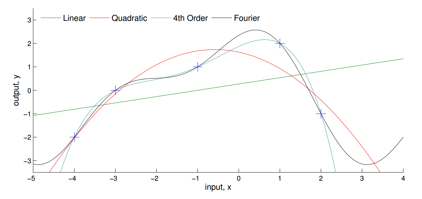
3. pre-specifying \(f(\textbf{X})\) may produce either overly complex or simple models
2. it's difficult to know a priori the most appropriate number of parameters
2. prespecifying the number of parameters, e.g \( \text{coefficients }\beta, \text{variance }\sigma^2 \)
1. it's difficult to know a priori the most appropriate function
Or
Bayesian Nonparametrics (2/2)
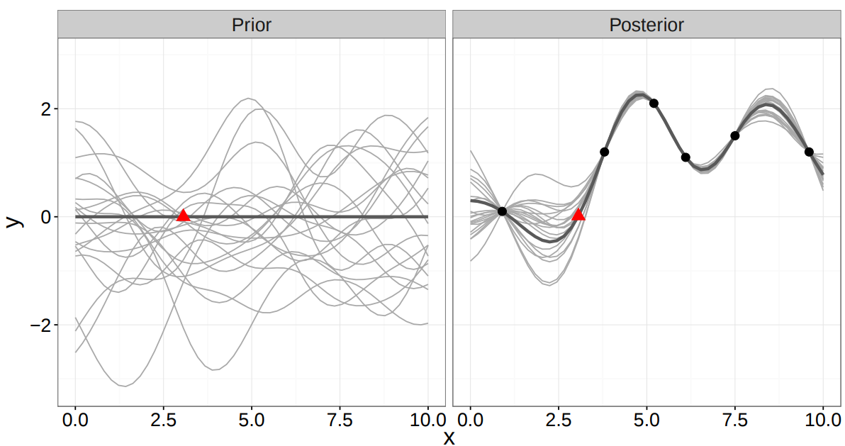
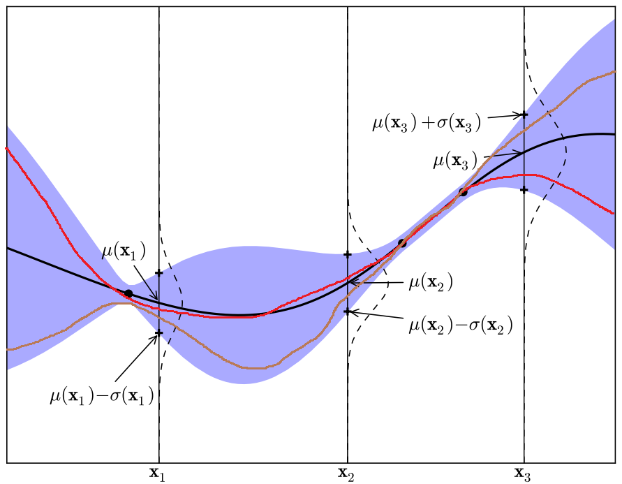
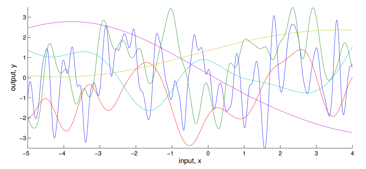
Gaussian Process
*Ghahramani, 2016
20
15
10
where
See Appendix for mathematical details
import pymc3 as pm

# Instantiate a model
with pm.Model() as latent_gp_model:

    # specify the priors
    length_scale = pm.Gamma("length_scale", alpha = 2, beta = 1)
    signal_variance = pm.HalfCauchy("signal_variance", beta = 5)
    noise_variance = pm.HalfCauchy("noise_variance", beta = 5)
    degrees_of_freedom = pm.Gamma("degrees_of_freedom", alpha = 2, beta = 0.1)

    # specify the kernel function
    cov = signal_variance**2 * pm.gp.cov.ExpQuad(1, length_scale)

    # specify the mean function
    mean_function = pm.gp.mean.Zero()

    # specify the gp
    gp = pm.gp.Latent(cov_func = cov)

    # specify the prior over the latent function
    f = gp.prior("f", X = X)

    # specify the likelihood
    obs = pm.StudentT("obs", mu = f, lam = 1/signal_variance, nu = degrees_of_freedom, observed = y)
# Perform Inference
with latent_gp_model:
    posterior = pm.sample(draws = 100, njobs = 2)
# extend the model by adding the GP conditional distribution so as to predict at test data
with latent_gp_model:
    f_pred = gp.conditional("f_pred", X_new)

# sample from the GP conditional posterior
with latent_gp_model:
    posterior_pred = pm.sample_ppc(posterior, vars = [f_pred], samples = 200)
Build a model
Train a model
Prediction
from sklearn.gaussian_process import GaussianProcessRegressor()

model = GaussianProcessRegressor()

model.fit(X_train, y_train)

model.predict(X_test, y_test)

model.score(X_test, y_test)

model.save('path/to/saved/model')
Few lines of code
from pmlearn.gaussian_process import GaussianProcessRegressor()

# Instantiate a PyMC3 Gaussian process model
model = GaussianProcessRegressor()

# Fit using MCMC or Variational Inference
model.fit(X_train, y_train)

model.predict(X_test, y_test)

model.score(X_test, y_test)

model.save('path/to/saved/model')
Few lines of code
import pymc3 as pm

# Instantiate a model
with pm.Model() as latent_gp_model:

    # specify the priors
    length_scale = pm.Gamma("length_scale", alpha = 2, beta = 1)
    signal_variance = pm.HalfCauchy("signal_variance", beta = 5)
    noise_variance = pm.HalfCauchy("noise_variance", beta = 5)
    degrees_of_freedom = pm.Gamma("degrees_of_freedom", alpha = 2, beta = 0.1)

    # specify the kernel function
    cov = signal_variance**2 * pm.gp.cov.ExpQuad(1, length_scale)

    # specify the mean function
    mean_function = pm.gp.mean.Zero()

    # specify the gp
    gp = pm.gp.Latent(cov_func = cov)

    # specify the prior over the latent function
    f = gp.prior("f", X = X)

    # specify the likelihood
    obs = pm.StudentT("obs", mu = f, lam = 1/signal_variance, nu = degrees_of_freedom, observed = y)


# Perform Inference
with latent_gp_model:
    posterior = pm.sample(draws = 100, njobs = 2)

# extend the model by adding the GP conditional distribution so as to predict at test data
with latent_gp_model:
    f_pred = gp.conditional("f_pred", X_new)

# sample from the GP conditional posterior
with latent_gp_model:
    posterior_pred = pm.sample_ppc(posterior, vars = [f_pred], samples = 200)
from pmlearn.gaussian_process import GaussianProcessRegressor()
# Instantiate a PyMC3 Gaussian process model
model = GaussianProcessRegressor()
# Fit using MCMC or Variational Inference
model.fit(X_train, y_train)
model.predict(X_test, y_test)Few lines of code
Many lines of code
PyMC3
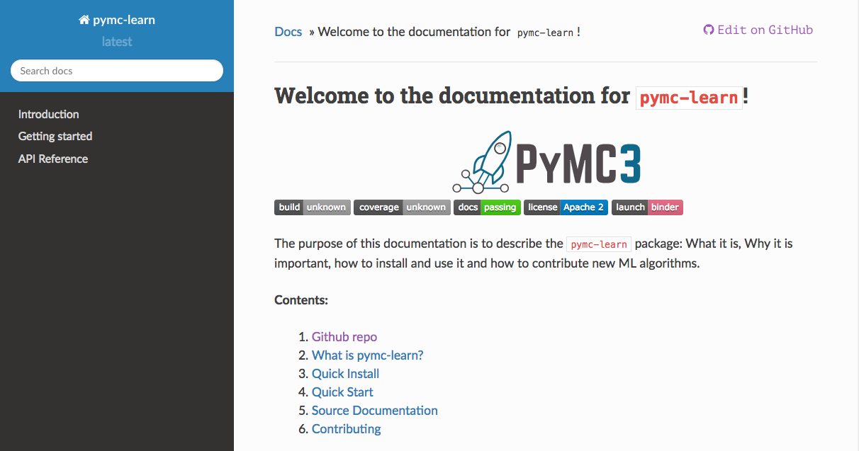
Pymc-learn
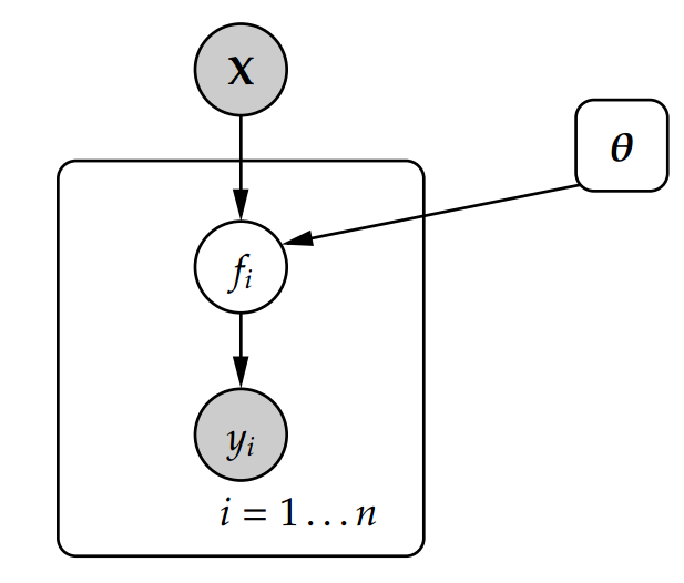
\(y_i\) = output variable,
\(\mathbf{x}_i\) = covariates with dimension \(D\), e.g {income, employment, trip distance, etc}
\(f(\mathbf{x}_i)\) = function that maps \(\mathbf{x}_i\) to \(y_i\),
\(\varepsilon_i\) = noise term,
\(p(\mathbf{\theta} \mid \textbf{y},\textbf{X})\) = posterior over the parameters, given observed data
\(p(\textbf{y} \mid \mathbf{\theta},\textbf{X})\) = likelihood of output variable, given covariates & parameters
\(p(\mathbf{\theta})\) = prior over the parameters
\(p(\textbf{y} \mid \textbf{X})\) = data distribution to ensure normalization
where
*Ghahramani, 2016; Williams & Rasmussen, 2006
\(p(\mathbf{f} \mid \textbf{y},\textbf{X})\) = posterior over the function, given observed data
\(p(\textbf{y} \mid \mathbf{f},\textbf{X})\) = likelihood of output variable, given the covariates & function
\(p(\mathbf{f})\) = prior over the function
\(p(\textbf{y} \mid \textbf{X})\) = data distribution to ensure normalization
*Ghahramani, 2016; Williams & Rasmussen, 2006
where
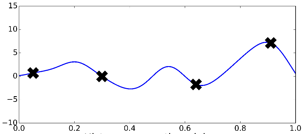
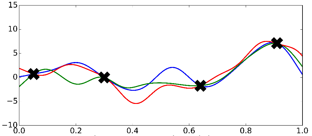
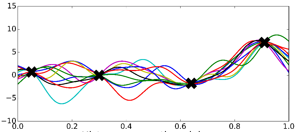
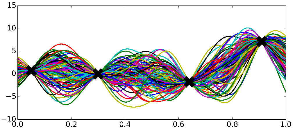
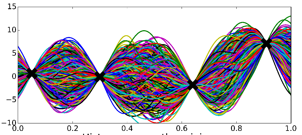
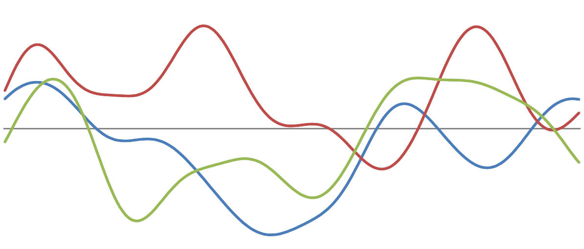
Very smooth i.e continuous
We expect our functions to vary smoothly
By Daniel Emaasit
Custom PyMC3 nonparametric Bayesian models built on top of the scikit-learn API


