Tools for Analysis and Visualization of Large Complex Data in R
Rencontres R
June 23, 2016
Follow along live: http://bit.ly/rr2015hafenv
View at your own pace: http://bit.ly/rr2015hafen
Packages to Install
install.packages(c("datadr", "trelliscope", "rbokeh"))(If you want to try it out - not required)
library(trelliscope)
library(rbokeh)
library(housingData)

panel <- function(x)
  figure() %>% ly_points(time, medListPriceSqft, data = x)
housing %>%
  qtrellis(by = c("county", "state"), panel, layout = c(2, 4))

# note: this will open up a web browser with a shiny app running
# use ctrl-c or esc to get back to your R prompt
To test the installation:
Background
Deep Analysis of Large Complex Data
Deep Analysis of
Large Complex Data
-
Data most often does not come with a model
-
If we already (think we) know the algorithm / model to apply and simply apply it to the data and do nothing else to assess validity, we are not doing analysis, we are processing
-
Deep analysis means detailed, comprehensive analysis that does not lose important information in the data
-
It means trial and error, an iterative process of hypothesizing, fitting, validating, learning
-
It means a lot of visualization
-
It means access to 1000s of statistical, machine learning, and visualization methods, regardless of data size
-
It means access to a high-level language to make iteration efficient
R is Great for Deep Analysis
-
Rapid prototyping
-
Access to 1000s of methods including excellent statistical visualization tools
-
Data structures and idioms tailored for data analysis
But R struggles with big data...
Deep Analysis of
Large Complex Data
Any or all of the following:
- Large number of records
- Many variables
- Complex data structures not readily put into tabular form of cases by variables
- Intricate patterns and dependencies that require complex models and methods of analysis
- Not i.i.d.!
Often complex data is more of a challenge than large data, but most large data sets are also complex
Goals
- Stay in R regardless of size of data
- Be able to use all methods available in R regardless of size of data
- Minimize both computation time (through scaling) and analyst time (through a simple interface in R) - with emphasis on analyst time
- Flexible data structures
- Scalable while keeping the same simple interface
Approach
Methodology:
Divide and Recombine
Software Implementation:
Tessera
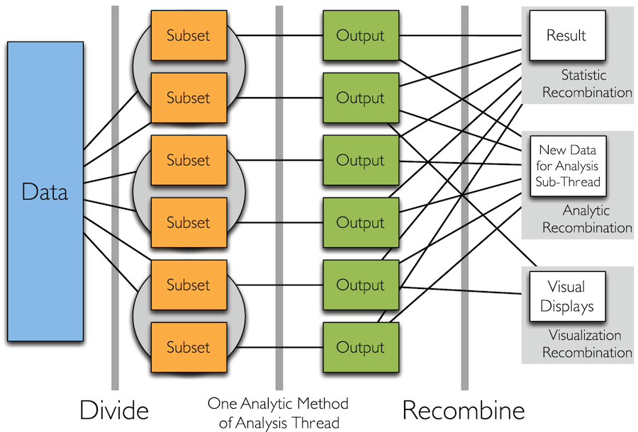
Divide and Recombine
Divide and Recombine
- Specify meaningful, persistent partioning of the data
- Analytic or visual methods are applied independently to each subset of the divided data in embarrassingly parallel fashion
- Results are recombined to yield a statistically valid D&R result for the analytic method
Simple Idea
Divide and Recombine
How to Divide the Data?
- Typically "big data" is big because it is made up of collections of smaller data from many subjects, sensors, locations, time periods, etc.
- It is therefore natural to break the data up based on these variables
- We call this conditioning variable division
- It is in practice by far the most common thing we do (and it's nothing new)
- Another option is random replicate division
Analytic Recombination
- Analytic recombination begins with applying an analytic method independently to each subset
- We can use any of the small-data methods we have available (think of the 1000s of methods in R)
- For conditioning-variable division:
- Typically the recombination depends on the subject matter
- Example: fit a linear model to each subset and combine the estimated coefficients for each subset to build a statistical model or for visual study
Analytic Recombination
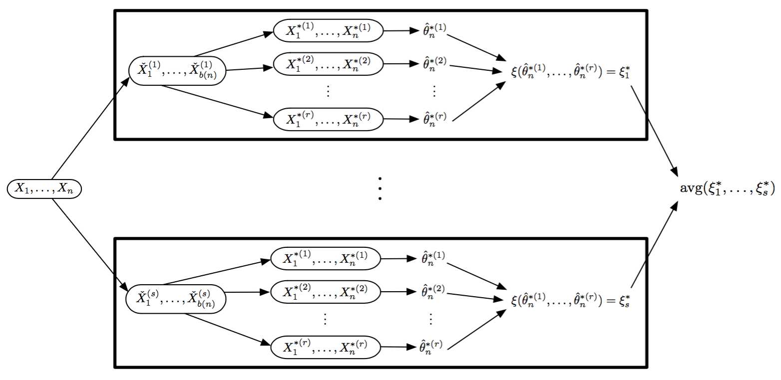
- For random replicate division:
- Division methods are based on statistical matters, not the subject matter as in conditioning-variable division
- Results are often approximations
- Approaches that fit this paradigm
- Coefficient averaging
- Subset likelihood modeling
- Bag of little bootstraps
- Consensus MCMC
Visual Recombination
-
Most visualization tools & approaches for big data either
- Summarize lot of data to create a single plot
- Are very specialized for a particular domain
- Summaries are critical
- But we must be able to flexibly visualize complex data in detail even when they are large!
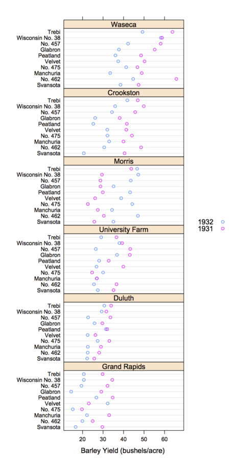
Trellis Display
- Data are split into meaningful subsets, usually conditioning on variables of the dataset
- A visualization method is applied to each subset
- The image for each subset is called a "panel"
- Panels are arranged in an array of rows, columns, and pages, resembling a garden trellis
Why Trellis is Effective
- Easy and flexible to create
- Data complexity / dimensionality can be handled by splitting the data up
- We have a great deal of freedom with what we plot inside each panel
- Easy and effective to consume
- Once a viewer understands one panel, they have immediate access to the data in all other panels
- Scanning across panels elicits comparisons to reveal repetition and change, pattern and surprise
Scaling Trellis
- Big data lends itself nicely to the idea of Trellis Display
- Recall that typically "big data" is big because it is made up of collections of smaller data from many subjects, sensors, locations, time periods, etc.
- It is natural to break the data up based on these dimensions and make a plot for each subset
- But this could mean Trellis displays with potentially thousands or millions of panels
- We can create millions of plots, but we will never be able to (or want to) view all of them!
Scaling Trellis
-
To scale, we can apply the same steps as in Trellis display, with one extra step:
- Data are split into meaningful subsets, usually conditioning on variables of the dataset
- A visualization method is applied to each subset
- A set of cognostics that measure attributes of interest for each subset is computed
- Panels are arranged in an array of rows, columns, and pages, resembling a garden trellis, with the arrangement being specified through interactions with the cognostics
Trelliscope is Scalable
- 6 months of US high frequency equity trading data
- Hundreds of gigabytes of data
- Split by stock symbol and day
- Nearly 1 million subsets
Tessera
An Implementation of D&R in R
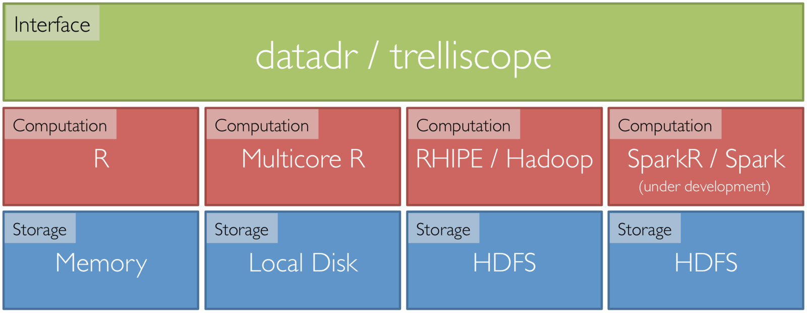
Tessera
Front end R packages that can tie to scalable back ends:
- datadr: an interface to data operations, division, and analytical recombination methods
- trelliscope: visual recombination through interactive multipanel exploration with cognostics
Data Structures in datadr
-
Must be able to break data down into pieces for independent storage / computation
-
Recall the potential for: “Complex data structures not readily put into tabular form of cases by variables”
-
Key-value pairs: a flexible storage paradigm for partitioned, distributed data
-
each subset of a division is an R list with two elements: key, value
-
keys and values can be any R object
-
# bySpecies <- divide(iris, by = "Species")

[[1]]
$key
  [1] "setosa"

$value
  Sepal.Length Sepal.Width Petal.Length Petal.Width
           5.1         3.5          1.4         0.2
           4.9         3.0          1.4         0.2
           4.7         3.2          1.3         0.2
           4.6         3.1          1.5         0.2
           5.0         3.6          1.4         0.2
  ...


[[2]]
$key
  [1] "versicolor"

$value
   Sepal.Length Sepal.Width Petal.Length Petal.Width
            7.0         3.2          4.7         1.4
            6.4         3.2          4.5         1.5
            6.9         3.1          4.9         1.5
            5.5         2.3          4.0         1.3
            6.5         2.8          4.6         1.5
  ...

[[3]]
$key
  [1] "virginica"

$value
  Sepal.Length Sepal.Width Petal.Length Petal.Width
           6.3         3.3          6.0         2.5
           5.8         2.7          5.1         1.9
           7.1         3.0          5.9         2.1
           6.3         2.9          5.6         1.8
           6.5         3.0          5.8         2.2
  ...
Example: Fisher's iris data
We can represent the data divided by species as a collection of key-value pairs
- Key is species name
- Value is a data frame of measurements for that species
Measurements in centimeters of the variables sepal length and width and petal length and width for 50 flowers from each of 3 species of iris: "setosa", "versicolor", and "virginica"
Each key-value pair is an independent unit and can be stored across disks, machines, etc.
[[1]]
$key
  [1] "setosa"

$value
  Sepal.Length Sepal.Width Petal.Length Petal.Width
           5.1         3.5          1.4         0.2
           4.9         3.0          1.4         0.2
           4.7         3.2          1.3         0.2
           4.6         3.1          1.5         0.2
           5.0         3.6          1.4         0.2
  ...


[[2]]
$key
  [1] "versicolor"

$value
   Sepal.Length Sepal.Width Petal.Length Petal.Width
            7.0         3.2          4.7         1.4
            6.4         3.2          4.5         1.5
            6.9         3.1          4.9         1.5
            5.5         2.3          4.0         1.3
            6.5         2.8          4.6         1.5
  ...

[[3]]
$key
  [1] "virginica"

$value
  Sepal.Length Sepal.Width Petal.Length Petal.Width
           6.3         3.3          6.0         2.5
           5.8         2.7          5.1         1.9
           7.1         3.0          5.9         2.1
           6.3         2.9          5.6         1.8
           6.5         3.0          5.8         2.2
  ...
Distributed Data Objects &
Distributed Data Frames
A collection of key-value pairs that forms a data set is called a distributed data object (ddo) and is the fundamental data type that is passed to and returned from most of the functions in datadr.
A ddo for which every value in each key value pair is a data frame of the same schema is called a distributed data frame (ddf)
This is a ddf (and a ddo)
[[1]]
$key
  [1] "setosa"

$value
  Call:
  loess(formula = Sepal.Length ~ Sepal.Width, data = x)

  Number of Observations: 50
  Equivalent Number of Parameters: 5.53
  Residual Standard Error: 0.2437

[[2]]
$key
  [1] "versicolor"

$value
  Call:
  loess(formula = Sepal.Length ~ Sepal.Width, data = x)

  Number of Observations: 50
  Equivalent Number of Parameters: 5
  Residual Standard Error: 0.4483

[[3]]
$key
  [1] "virginica"

$value
  Call:
  loess(formula = Sepal.Length ~ Sepal.Width, data = x)

  Number of Observations: 50
  Equivalent Number of Parameters: 5.59
  Residual Standard Error: 0.5683
Distributed Data Objects &
Distributed Data Frames
Suppose we fit a loess model to each subset and store the result in a new collection of key-value pairs.
This is a ddo but not a ddf
datadr Data Connections
-
Distributed data types / backend connections
-
localDiskConn(), hdfsConn() connections to ddo / ddf objects persisted on a backend storage system
-
ddo(): instantiate a ddo from a backend connection
-
ddf(): instantiate a ddf from a backend connection
-
-
Conversion methods between data stored on different backends
Computation in datadr
MapReduce
-
A general-purpose paradigm for processing big data sets
-
The standard processing paradigm in Hadoop
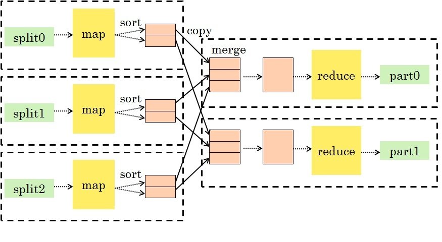
MapReduce
- Map: take input key-value pairs and apply a map function, emitting intermediate transformed key-value pairs
-
Shuffle: group map outputs by intermediate key
-
Reduce: for each unique intermediate key, gather all values and process with a reduce function
This is a very general and scalable approach to processing data.
MapReduce Example
- Map: for each species in the input key-value pair, emit the species as the key and the max as the value
- Reduce: for each grouped intermediate species key, compute the maximum of the values
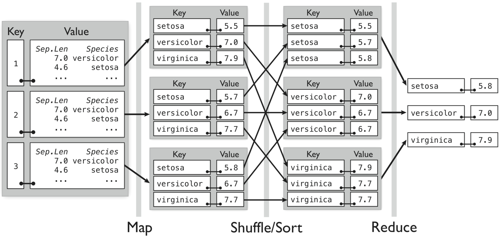
Compute maximum sepal length by species for randomly divided iris data
MapReduce Example
maxMap <- expression({
  # map.values: list of input values
  for(v in map.values) {
    # v is a data.frame
    # for each species, "collect" a
    # k/v pair to be sent to reduce
    by(v, v$Species, function(x) {
      collect(
        x$Species[1],       # key
        max(x$Sepal.Length) # value
      )
    })
  }
})
Map
# reduce is called for unique intermediate key
# "pre" is an initialization called once
# "reduce" is called for batches of reduce.values
# "post" runs after processing all reduce.values
maxReduce <- expression(
  pre={
    speciesMax <- NULL
  },
  reduce={
    curValues <- do.call(c, reduce.values)
    speciesMax <- max(c(speciesMax, curValues))
  },
  post={
    collect(reduce.key, speciesMax)
  }
)
Reduce
This may not look very intuitive
But could be run on hundreds of terabytes of data
And it's much easier than what you'd write in Java
Computation in datadr
- Everything uses MapReduce under the hood
-
As often as possible, functions exist in datadr to shield the analyst from having to write MapReduce code
MapReduce is sufficient
for all D&R operations
D&R methods in datadr
-
A divide() function takes a ddf and splits it using conditioning or random replicate division
-
Analytic methods are applied to a ddo/ddf with the addTransform() function
-
Recombinations are specified with recombine(), which provides some standard combiner methods, such as combRbind(), which binds transformed results into single data frame
-
Division of ddos with arbitrary data structures must typically be done with custom MapReduce code (unless data can be temporarily transformed into a ddf)
datadr Other Data Operations
-
drLapply(): apply a function to each subset of a ddo/ddf and obtain a new ddo/ddf
-
drJoin(): join multiple ddo/ddf objects by key
-
drSample(): take a random sample of subsets of a ddo/ddf
-
drFilter(): filter out subsets of a ddo/ddf that do not meet a specified criteria
-
drSubset(): return a subset data frame of a ddf
-
drRead.table() and friends
-
mrExec(): run a traditional MapReduce job on a ddo/ddf
datadr Division Independent Methods
-
drQuantile(): estimate all-data quantiles, optionally by a grouping variable
-
drAggregate(): all-data tabulation
-
drHexbin(): all-data hexagonal binning aggregation
-
summary() method computes numerically stable moments, other summary stats (freq table, range, #NA, etc.)
-
More to come
Scalable Setup
Set up your own Hadoop cluster:
http://tessera.io/docs-install-cluster/
Set up a cluster on Amazon Web Services:
./tessera-emr.sh -n 10 -s s3://tessera-emr -m m3.xlarge -w m3.xlarge
What's Different About Tessera?
- Restrictive in data structures (only data frames / tabular / matrix algebra)
- Restrictive in methods (only SQL-like operations or a handful of scalable non-native algorithms)
- Or both!
Many other "big data" systems that support R are either:
Idea of Tessera:
- Let's use R for the flexibility it was designed for, regardless of the size of the data
- Use any R data structure and run any R code at scale
More Information
- website: http://tessera.io
- code: http://github.com/tesseradata
- Twitter: @TesseraIO
- Google user group
-
Try it out
- If you have some applications in mind, give it a try!
- You don’t need big data or a cluster to use Tessera
- Ask us for help, provide feedback, join in
For more information (docs, code, papers, user group, blog, etc.): http://tessera.io
Tangent 1: http://hafen.github.io/rbokeh/
Tangent 2: http://gallery.htmlwidgets.org/
Thank You
Small Data Example You Can Experiment With
US Home Prices by State and County from Zillow
Zillow Housing Data
- Housing sales and listing data in the United States
- Between 2008-10-01 and 2014-03-01
- Aggregated to the county level
- Zillow.com data provided by Quandl
library(housingData)

head(housing)

#    fips         county state       time nSold medListPriceSqft medSoldPriceSqft
# 1 06001 Alameda County    CA 2008-10-01    NA         307.9787         325.8118
# 2 06001 Alameda County    CA 2008-11-01    NA         299.1667               NA
# 3 06001 Alameda County    CA 2008-11-01    NA               NA         318.1150
# 4 06001 Alameda County    CA 2008-12-01    NA         289.8815         305.7878
# 5 06001 Alameda County    CA 2009-01-01    NA         288.5000         291.5977
# 6 06001 Alameda County    CA 2009-02-01    NA         287.0370               NA
Housing Data Variables
| Variable | Description |
|---|---|
| fips | Federal Information Processing Standard - a 5 digit county code |
| county | US county name |
| state | US state name |
| time | date (the data is aggregated monthly) |
| nSold | number sold this month |
| medListPriceSqft | median list price per square foot (USD) |
| medSoldPriceSqft | median sold price per square foot (USD) |
Data Ingest
- When working with any data set, the first thing to do is create a ddo/ddf from the data
You Try It
Our housing data is already in memory, so we can use the simple approach of casting the data frame as a ddf:
library(datadr)
library(housingData)

housingDdf <- ddf(housing)
# print result to see what it looks like
housingDdf
# Distributed data frame backed by 'kvMemory' connection
#
# attribute | value
# ----------------+----------------------------------------------------------------
# names | fips(fac), county(fac), state(fac), time(Dat), and 3 more
# nrow | 224369
# size (stored) | 10.58 MB
# size (object) | 10.58 MB
# # subsets | 1
#
# * Other attributes: getKeys()
# * Missing attributes: splitSizeDistn, splitRowDistn, summaryDivide by county and state
One useful way to look at the data is divided by county and state
byCounty <- divide(housingDdf,
    by = c("county", "state"), update = TRUE)
* update = TRUE tells datadr to compute and update the attributes of the ddf (seen in printout)
byCounty

# Distributed data frame backed by 'kvMemory' connection
#
#  attribute      | value
# ----------------+----------------------------------------------------------------
#  names          | fips(cha), time(Dat), nSold(num), and 2 more
#  nrow           | 224369
#  size (stored)  | 15.73 MB
#  size (object)  | 15.73 MB
#  # subsets      | 2883
#
# * Other attributes: getKeys(), splitSizeDistn(), splitRowDistn(), summary()
# * Conditioning variables: county, state
Investigating the ddf
Recall that a ddf is a collection of key-value pairs
# look at first key-value pair
byCounty[[1]]

# $key
# [1] "county=Abbeville County|state=SC"
#
# $value
#    fips       time nSold medListPriceSqft medSoldPriceSqft
# 1 45001 2008-10-01    NA         73.06226               NA
# 2 45001 2008-11-01    NA         70.71429               NA
# 3 45001 2008-12-01    NA         70.71429               NA
# 4 45001 2009-01-01    NA         73.43750               NA
# 5 45001 2009-02-01    NA         78.69565               NA
# ...
Investigating the ddf
# look at first two key-value pairs
byCounty[1:2]

# [[1]]
# $key
# [1] "county=Abbeville County|state=SC"#
#
# $value
#    fips       time nSold medListPriceSqft medSoldPriceSqft
# 1 45001 2008-10-01    NA         73.06226               NA
# 2 45001 2008-11-01    NA         70.71429               NA
# 3 45001 2008-12-01    NA         70.71429               NA
# 4 45001 2009-01-01    NA         73.43750               NA
# 5 45001 2009-02-01    NA         78.69565               NA
# ...#
#
#
# [[2]]
# $key
# [1] "county=Acadia Parish|state=LA"#
#
# $value
#    fips       time nSold medListPriceSqft medSoldPriceSqft
# 1 22001 2008-10-01    NA         67.77494               NA
# 2 22001 2008-11-01    NA         67.16418               NA
# 3 22001 2008-12-01    NA         63.59129               NA
# 4 22001 2009-01-01    NA         65.78947               NA
# 5 22001 2009-02-01    NA         65.78947               NA
# ...
Investigating the ddf
# lookup by key
byCounty[["county=Benton County|state=WA"]]

# $key
# [1] "county=Benton County|state=WA"
#
# $value
#    fips       time nSold medListPriceSqft medSoldPriceSqft
# 1 53005 2008-10-01   137         106.6351         106.2179
# 2 53005 2008-11-01    80         106.9650               NA
# 3 53005 2008-11-01    NA               NA         105.2370
# 4 53005 2008-12-01    95         107.6642         105.6311
# 5 53005 2009-01-01    73         107.6868         105.8892
# ...
You Try It
Try using the divide statement to divide on one or more variables
press down arrow key for solution when you're ready
Possible Solutions
byState <- divide(housing, by="state")

byMonth <- divide(housing, by="time")
ddf Attributes
summary(byCounty)

#         fips                 time                nSold
#  -------------------  ------------------  -------------------
#        levels : 2883  missing :        0   missing :   164370
#       missing : 0         min : 08-10-01       min :       11
#  > freqTable head <       max : 14-03-01       max :    35619
#  26077 : 140                                  mean : 274.6582
#  51069 : 140                               std dev : 732.2429
#  08019 : 139                              skewness :   10.338
#  13311 : 139                              kurtosis : 222.8995
#  -------------------  ------------------  -------------------
# ...

names(byCounty)

# [1] "fips"             "time"             "nSold"            "medListPriceSqft"
# [5] "medSoldPriceSqft"

length(byCounty)

# [1] 2883

getKeys(byCounty)

# [[1]]
# [1] "county=Abbeville County|state=SC"
# ...
Transformations
-
addTransform(data, fun) applies a function fun to each value of a key-value pair in the input ddo/ddf data
-
e.g. calculate a summary statistic for each subset
-
-
The transformation is not applied immediately, it is deferred until:
-
A function that kicks off a MapReduce job is called, e.g. recombine()
-
A subset of the data is requested (e.g. byCounty[[1]])
-
The drPersist() function explicitly forces transformation computation to persist
-
Transformation Example
Compute the slope of a simple linear regression of list price vs. time
# function to calculate a linear model and extract the slope parameter
lmCoef <- function(x) {
  coef(lm(medListPriceSqft ~ time, data = x))[2]
}

# best practice tip: test transformation function on one subset
lmCoef(byCounty[[1]]$value)

#          time
# -0.0002323686

# apply the transformation function to the ddf
byCountySlope <- addTransform(byCounty, lmCoef)
Transformation example
# look at first key-value pair
byCountySlope[[1]]

# $key
# [1] "county=Abbeville County|state=SC"
#
# $value
#          time
# -0.0002323686

# what does this object look like?
byCountySlope

# Transformed distributed data object backed by 'kvMemory' connection
#
#  attribute      | value
# ----------------+----------------------------------------------------------------
#  size (stored)  | 15.73 MB (before transformation)
#  size (object)  | 15.73 MB (before transformation)
#  # subsets      | 2883
#
# * Other attributes: getKeys()
# * Conditioning variables: county, state
*note: this is a ddo (value isn't a data frame) but it is still pointing to byCounty's data
Exercise: create a transformation function
Create a new transformed data set using addTransform()
- Add/remove/modify variables
- Compute a summary (# rows, #NA, etc.)
- etc.
# get a subset
x <- byCounty[[1]]$value

# now experiment with x and stick resulting code into a transformation function

# some scaffolding for your solution:
transformFn <- function(x) {
  ## you fill in here
}

xformedData <- addTransform(byCounty, transformFn)
Hint: it is helpful to grab a subset and experiment with it and then stick that code into a function:
Possible Solutions
# example 1 - total sold over time for the county
totalSold <- function(x) {
   sum(x$nSold, na.rm=TRUE)
}
byCountySold <- addTransform(byCounty, totalSold)

# example 2 - range of time for which data exists for county
timeRange <- function(x) {
   range(x$time)
}
byCountyTime <- addTransform(byCounty, timeRange)

# example 3 - convert usd/sqft to euro/meter
us2eur <- function(x)
  x * 2.8948

byCountyEur <- addTransform(byCounty, function(x) {
  x$medListPriceMeter <- us2eur(x$medListPriceSqft)
  x$medSoldPriceMeter <- us2eur(x$medSoldPriceSqft)
  x
})
Note that the us2eur function was detected - this becomes useful in distributed computing when shipping code across many computers
Recombination
countySlopes <- recombine(byCountySlope, combine = combRbind)Let's recombine the slopes of list price vs. time into a data frame.
This is an example of statistic recombination where the result is small and is pulled back into R for further investigation.
head(countySlopes)

#           county state           val
# Abbeville County    SC -0.0002323686
#    Acadia Parish    LA  0.0019518441
#  Accomack County    VA -0.0092717711
#       Ada County    ID -0.0030197554
#     Adair County    IA -0.0308381951
#     Adair County    KY  0.0034399585
Recombination Options
-
combine parameter controls the form of the result
-
combine=combRbind: rbind is used to combine all of the transformed key-value pairs into a local data frame in your R session - this is a frequently used option
-
combine=combCollect: transformed key-value pairs are collected into a local list in your R session
-
combine=combDdo: results are combined into a new ddo object
-
Others can be written for more sophisticated goals such as model coefficient averaging, etc.
-
Persisting a Transformation
us2eur <- function(x)
  x * 2.8948

byCountyEur <- addTransform(byCounty, function(x) {
  x$medListPriceMeter <- us2eur(x$medListPriceSqft)
  x$medSoldPriceMeter <- us2eur(x$medSoldPriceSqft)
  x
})

byCountyEur <- drPersist(byCountyEur)
Often we want to persist a transformation, creating a new ddo or ddf that contains the transformed data. Transforming and persisting a transformation is an analytic recombination.
Let's persist the US/sqft to EUR/sqmeter transformation using drPersist():
*note we can also use recombine(combine = combDdf) - drPersist() is for convenience
Joining Multiple Datasets
We have a few additional data sets we'd like to join with our home price data divided by county
head(geoCounty)

#    fips         county state       lon      lat rMapState rMapCounty
# 1 01001 Autauga County    AL -86.64565 32.54009   alabama    autauga
# 2 01003 Baldwin County    AL -87.72627 30.73831   alabama    baldwin
# 3 01005 Barbour County    AL -85.39733 31.87403   alabama    barbour
# 4 01007    Bibb County    AL -87.12526 32.99902   alabama       bibb
# 5 01009  Blount County    AL -86.56271 33.99044   alabama     blount
# 6 01011 Bullock County    AL -85.71680 32.10634   alabama    bullock

head(wikiCounty)

#    fips         county state pop2013                                                 href
# 1 01001 Autauga County    AL   55246 http://en.wikipedia.org/wiki/Autauga_County,_Alabama
# 2 01003 Baldwin County    AL  195540 http://en.wikipedia.org/wiki/Baldwin_County,_Alabama
# 3 01005 Barbour County    AL   27076 http://en.wikipedia.org/wiki/Barbour_County,_Alabama
# 4 01007    Bibb County    AL   22512    http://en.wikipedia.org/wiki/Bibb_County,_Alabama
# 5 01009  Blount County    AL   57872  http://en.wikipedia.org/wiki/Blount_County,_Alabama
# 6 01011 Bullock County    AL   10639 http://en.wikipedia.org/wiki/Bullock_County,_Alabama
Exercise: Divide by County and State
- To join these with our byCounty data set, we first must divide by county and state
- Give it a try:
byCountyGeo <- # ...

byCountyWiki <- # ...
Exercise: Divide by County and State
byCountyGeo <- divide(geoCounty,
  by=c("county", "state"))

byCountyWiki <- divide(wikiCounty,
  by=c("county", "state"))
byCountyGeo
# Distributed data frame backed by 'kvMemory' connection
#
# attribute | value
# ----------------+----------------------------------------------------------------
# names | fips(cha), lon(num), lat(num), rMapState(cha), rMapCounty(cha)
# nrow | 3075
# size (stored) | 8.14 MB
# size (object) | 8.14 MB
# # subsets | 3075
# ...byCountyGeo[[1]]
# $key
# [1] "county=Abbeville County|state=SC"
#
# $value
# fips lon lat rMapState rMapCounty
# 1 45001 -82.45851 34.23021 south carolina abbevilleJoining the Data
drJoin() takes any number of named parameters specifying ddo/ddf objects and returns a ddo of the objects joined by key
joinedData <- drJoin(
  housing = byCountyEur,
  slope   = byCountySlope,
  geo     = byCountyGeo,
  wiki    = byCountyWiki)
joinedData
# Distributed data object backed by 'kvMemory' connection
#
# attribute | value
# ----------------+----------------------------------------------------------------
# size (stored) | 29.23 MB
# size (object) | 29.23 MB
# # subsets | 3144
Joining the Data
What does this object look like?
str(joinedData[[1]])

# List of 2
#  $ key  : chr "county=Abbeville County|state=SC"
#  $ value:List of 4
#   ..$ housing:'data.frame': 66 obs. of  7 variables:
#   .. ..$ fips             : chr [1:66] "45001" "45001" "45001" "45001" ...
#   .. ..$ time             : Date[1:66], format: "2008-10-01" "2008-11-01" ...
#   .. ..$ nSold            : num [1:66] NA NA NA NA NA NA NA NA NA NA ...
#   .. ..$ medListPriceSqft : num [1:66] 73.1 70.7 70.7 73.4 78.7 ...
#   .. ..$ medSoldPriceSqft : num [1:66] NA NA NA NA NA NA NA NA NA NA ...
#   .. ..$ medListPriceMetre: num [1:66] 1114 1078 1078 1120 1200 ...
#   .. ..$ medSoldPriceMetre: num [1:66] NA NA NA NA NA NA NA NA NA NA ...
#   ..$ slope  : Named num -0.000232
#   ..$ geo    :'data.frame': 1 obs. of  5 variables:
#   .. ..$ fips      : chr "45001"
#   .. ..$ lon       : num -82.5
#   .. ..$ lat       : num 34.2
#   .. ..$ rMapState : chr "south carolina"
#   .. ..$ rMapCounty: chr "abbeville"
#   ..$ wiki   :'data.frame': 1 obs. of  3 variables:
#   .. ..$ fips   : chr "45001"
#   .. ..$ pop2013: int 25007
#   .. ..$ href   : chr "http://en.wikipedia.org/wiki/Abbeville_County,_South Carolina"
# ...
for a given county/state, the value is a list with elements according to data provided in drJoin()
Joined Data
Note that joinedData has more subsets than byCountyEur
length(byCountyEur)

# [1] 2883

length(joinedData)

# [1] 3144- Some of the data sets we joined have more counties than we have data for in byCountyEur
- drJoin() makes a subset for every unique key across all input data sets
- If data is missing in a subset, it doesn't have an entry
# Adams County Iowa only has geo and wiki data
joinedData[["county=Adams County|state=IA"]]$value

# $geo
#    fips       lon      lat rMapState rMapCounty
# 1 19003 -94.70909 41.03166      iowa      adams
#
# $wiki
#    fips pop2013                                            href
# 1 19003    3894 http://en.wikipedia.org/wiki/Adams_County,_Iowa
Bonus Problem
Can you write a transformation and recombination to get all counties for which joinedData does not have housing information?
Solution
noHousing <- joinedData %>%
  addTransform(function(x) is.null(x$housing)) %>%
  recombine(combRbind)

head(subset(noHousing, val == TRUE))

#               county state  val
# 2884    Adams County    IA TRUE
# 2885    Adams County    ND TRUE
# 2886 Antelope County    NE TRUE
# 2887   Arthur County    NE TRUE
# 2888   Ashley County    AR TRUE
# 2889   Aurora County    SD TRUE
tx <- addTransform(joinedData, function(x) is.null(x$housing))
noHousing <- recombine(tx, combRbind)(without pipes)
Filtering
Suppose we only want to keep subsets of joinedData that have housing price data
- drFilter(data, fun) applies a function fun to each value of a key-value pair in the input ddo/ddf data
- If fun returns TRUE we keep the key-value pair
joinedData <- drFilter(joinedData,
  function(x) {
    !is.null(x$housing)
  })
# joinedData should now have as many subsets as byCountyAus
length(joinedData)
# [1] 2883Trelliscope
- We now have a ddo, joinedData, which contains pricing data as well as a few other pieces of information like geographic location and a link to wikipedia for 2,883 counties in the US
- Using this data, let's make a simple plot of list price vs. time for each county and put it in a Trelliscope display
Trelliscope Setup
- Trelliscope stores its displays in a "Visualization Database" (VDB), which is a collection of files on your disk that contain metadata about the displays
- To create and view displays, we must first establish a connection to the VDB
library(trelliscope)

# establish a connection to a VDB located in a directory "housing_vdb"
vdbConn("housing_vdb", name = "housingexample")- If this location has not already been initialized as a VDB, you will be prompted if you want to create one at this location (you can set autoYes = TRUE to skip the prompt)
- If it has been initialized, it will simply make the connection
Trelliscope Display Fundamentals
- A Trelliscope display is created with the function makeDisplay()
- At a minimum, a specification of a Trelliscope display must have the following:
- data: a ddo or ddf input data set
- name: the name of the display
- panelFn: a function that operates on the value of each key-value pair and produces a plot
- There are several other options, some of which we will see and some of which you can learn more about in the documentation
A Simple Panel Function
Plot list price vs. time using rbokeh
library(rbokeh)

timePanel <- function(x) {
  xlim <- c("2008-07-01", "2014-06-01")

  figure(ylab = "Price / Sq. Meter (EUR)",
    xlim = as.Date(xlim)) %>%
  ly_points(time, medListPriceMeter,
    data = x$housing,
    hover = list(time, medListPriceMeter))
}

# test it on a subset
timePanel(joinedData[[1]]$value)
Make a Display
makeDisplay(joinedData,
  name = "list_vs_time_rbokeh",
  desc = "List price over time for each county.",
  panelFn = timePanel
)
- This creates a display and adds its meta data to the directory we specified in vdbConn()
- We can view the display with this:
view()

# to go directly to this display
view("list_vs_time_rbokeh")
Try Your Own Panel Function
Ideas: recreate the previous plot with your favorite plotting package, or try something new (histogram of prices, etc.)
Make a panel function,
test it,
and make a new display with it
Possible Solutions
library(lattice)
library(ggplot2)

latticeTimePanel <- function(x) {
  xyplot(medListPriceMeter + medSoldPriceMeter ~ time,
    data = x$housing, auto.key = TRUE,
    ylab = "Price / Meter (EUR)")
}

makeDisplay(joinedData,
  name = "list_vs_time_lattice",
  desc = "List price over time for each county.",
  panelFn = latticeTimePanel
)

ggTimePanel <- function(x) {
  qplot(time, medListPriceMeter, data = x$housing,
    ylab = "Price / Meter (EUR)") +
  geom_point()
}

makeDisplay(joinedData,
  name = "list_vs_time_ggplot2",
  desc = "List price over time for each county.",
  panelFn = ggTimePanel
)
A Display with Cognostics
- The interactivity in these examples hasn't been too interesting
- We can add more interactivity through cognostics
- Like the panel function, we can supply a cognostics function that
- Takes a subset of the data as input and returns a named list of summary statistics or cognostics about the subset
- A helper function cog() can be used to supply additional attributes like descriptions to help the viewer understand what the cognostic is
- These can be used for enhanced interaction with the display, helping the user focus their attention on panels of interest
Cognostics Function
zillowCog <- function(x) {
  # build a string for a link to zillow
  st <- getSplitVar(x, "state")
  ct <- getSplitVar(x, "county")
  zillowString <- gsub(" ", "-", paste(ct, st))

  # return a list of cognostics
  list(
    slope = cog(x$slope, desc = "list price slope"),
    meanList = cogMean(x$housing$medListPriceMeter),
    meanSold = cogMean(x$housing$medSoldPriceMeter),
    lat = cog(x$geo$lat, desc = "county latitude"),
    lon = cog(x$geo$lon, desc = "county longitude"),
    wikiHref = cogHref(x$wiki$href, desc="wiki link"),
    zillowHref = cogHref(
      sprintf("http://www.zillow.com/homes/%s_rb/", zillowString),
      desc="zillow link")
  )
}
# test it on a subset
zillowCog(joinedData[[1]]$value)
# $slope
# time
# -0.0002323686
#
# $meanList
# [1] 1109.394
#
# $meanSold
# [1] NaN
#
# $lat
# [1] 34.23021
#
# $lon
# [1] -82.45851
#
# $wikiHref
# [1] "<a href=\"http://en.wikipedia.org/wiki/Abbeville_County,_South Carolina\" target=\"_blank\">link</a>"
#
# $zillowHref
# [1] "<a href=\"http://www.zillow.com/homes/Abbeville-County-SC_rb/\" target=\"_blank\">link</a>"
Display with Cognostics
We simply add our cognostics function to makeDisplay()
makeDisplay(joinedData,
  name = "list_vs_time_cog",
  desc = "List price over time for each county.",
  panelFn = timePanel,
  cogFn = zillowCog
)
Rencontres R 2016
By Ryan Hafen


