A gentle introduction to Particle Filters

EA503 - DSP - Prof. Luiz Eduardo

Agenda
- Tools from statistics + Recap
- Particle filters and its components
- An algorithm (In Python)
Classical statistics
We place probability distributions on data
(only data is random)
Bayesian statistics
We place probability distributions in the model and in parameters
Probability represents uncertainty
P(Hypothesis|Data)
Posterior
Probability
P(Data|Hypothesis)
Likelihood
P(Hypothesis)
Prior
Bayesian statistics
P(Hypothesis|Data) = \frac{P(Hypothesis)*P(Data|Hypothesis)}{P(Data)}
Recursively,
P(Hypothesis|Data) = P(H_t|H_{t-1}, D_t)
Bayesian statistics
P(Hypothesis|Data) = P(H_t|H_{t-1}, D_t)

Every time we get a new step, we should be able to improve our state estimation
Kalman Filter
P(H_t|H_{t-1}, A_t, D_t)
Prediction + correction
Constraint: It needs to be a Gaussian distribution
It is also a recursive structure
Can we represent these recursive models as chains?
X_{t-1}
X_{t}
X_{t+1}
Markov chain
X is the true information
P(X_t|X_{t-1})
We may not have access to the true information, but to a measured (estimated) value
X_{t-1}
X_{t}
X_{t+1}
Y_{t-1}
Y_{t}
Y_{t+1}
Hidden Markov chain
P(Y_t|X_{t})
X_{t-1}
X_{t}
X_{t+1}
Y_{t-1}
Y_{t}
Y_{t+1}
What can we say about this model in terms of P?
X_{t-1}
X_{t}
X_{t+1}
Y_{t-1}
Y_{t}
Y_{t+1}
Goal:
P(X_t|Y_1,...,Y_{t})
Consider all the observations for the estimation
[marginal distribution]
Goal:
P(X_t|Y_1,...,Y_{t})
We know
P(X_t|X_{t-1})
P(Y_t|X_{t})
and
Considering that this is a recursive process,
P(X_{t-1}|Y_1,...,Y_{t-1})
Combining these Probabilities:
P(Y_{t},X_{t},X_{t-1}|Y_1,...,Y_{t-1})
Goal:
P(X_t|Y_1,...,Y_{t})
We know
P(X_t|X_{t-1})
P(Y_t|X_{t})
and
Considering that this is a recursive process,
P(X_{t-1}|Y_1,...,Y_{t-1})
Combining these Probabilities:
P(Y_{t},X_{t},X_{t-1}|Y_1,...,Y_{t-1})
Goal:
P(X_t|Y_1,...,Y_{t})
We know
P(X_t|X_{t-1})
P(Y_t|X_{t})
and
Considering that this is a recursive process,
P(X_{t-1}|Y_1,...,Y_{t-1})
Combining these Probabilities:
P(Y_{t},X_{t},X_{t-1}|Y_1,...,Y_{t-1})
Goal:
P(X_t|Y_1,...,Y_{t})
We know
P(X_t|X_{t-1})
P(Y_t|X_{t})
and
Considering that this is a recursive process,
P(X_{t-1}|Y_1,...,Y_{t-1})
Combining these Probabilities:
P(Y_{t},X_{t},X_{t-1}|Y_1,...,Y_{t-1})
Not
Relevant in this formula
Goal:
P(X_t|Y_1,...,Y_{t})
In a particular point,
P(Y_{t}=y,X_{t},X_{t-1}=x|Y_1,...,Y_{t-1})
Sum x (it'll remove )
X_{t-1}
\sum_{x} P(Y_{t}=y,X_{t},X_{t-1}=x|Y_1,...,Y_{t-1})
P(Y_{t}=y,X_{t}|Y_1,...,Y_{t-1}) =
Goal:
P(X_t|Y_1,...,Y_{t})
Get rid of
Y_{t} = y
\sum_{x} P(Y_{t}=y,X_{t}=x|Y_1,...,Y_{t-1})
P(Y_{t}=y,X_{t}|Y_1,...,Y_{t-1})
Current:
Another manipulation
P(Y_{t}=y|Y_1,...,Y_{t-1}) =
Goal:
P(X_t|Y_1,...,Y_{t})
\frac{P(Y_{t}=y,X_{t}|Y_1,...,Y_{t-1})}{\sum_{x} P(Y_{t}=y,X_{t}=x|Y_1,...,Y_{t-1})}
Final
arrangement:
And this is the set of ideas we need for understanding...
[joint distribution]
Agenda
- Tools from statistics + Recap
- Particle filters and its components
- An algorithm (In Python)
Goal:
P(X_t|Y_1,...,Y_{t})
\frac{P(Y_{t}=y,X_{t}|Y_1,...,Y_{t-1})}{\sum_{x} P(Y_{t}=y,X_{t}=x|Y_1,...,Y_{t-1})}
Final
arrangement:
This computation can be REALLY heavy (O^2)
[joint distribution]
Let's use points (particles) to represent our space
Let's estimate this joint distribution as a sum of weighted trajectories of this particles
Goal:
P(X_t|Y_1,...,Y_{t})
\frac{P(Y_{t}=y,X_{t}|Y_1,...,Y_{t-1})}{\sum_{x} P(Y_{t}=y,X_{t}=x|Y_1,...,Y_{t-1})}
Final
arrangement:

In pictures
Goal:
P(X_t|Y_1,...,Y_{t})
\frac{P(Y_{t}=y,X_{t}|Y_1,...,Y_{t-1})}{\sum_{x} P(Y_{t}=y,X_{t}=x|Y_1,...,Y_{t-1})}
Final
arrangement:
In pictures

Goal:
P(X_t|Y_1,...,Y_{t})
\frac{P(Y_{t}=y,X_{t}|Y_1,...,Y_{t-1})}{\sum_{x} P(Y_{t}=y,X_{t}=x|Y_1,...,Y_{t-1})}
Final
arrangement:
In formulas
\frac{P(Y_{t}=y,X_{t}|Y_1,...,Y_{t-1})}{\sum_{x} P(Y_{t}=y,X_{t}=x|Y_1,...,Y_{t-1})} \overset{\Delta}{=}
\sum_{i=1}^{NumParticles} weight^{i} \delta(X_{t-1} - X_{t}^i)
The sum of these weights is 1
The joint distribution becomes a sum of impulses with weights
The weight is proportional to three components:
1.
P(Y_{t}|X_{t})
Observation probability
2.
P(X_{t}|X_{t-1}=x)
Transition probability
3.
P(X_{t}|X_{t-1}=x_0,Y_1,...,Y_{t-1})
Computation
from previous step
We can build a recursive formula for the weight of a given particle i
P(Y_{t}|X_{t})
P(X_{t}|X_{t-1}=x)
P(X_{t}|X_{t-1}=x_0,Y_1,...,Y_{t-1})
w_{t}^{i} =
w_{t-1}^{i}
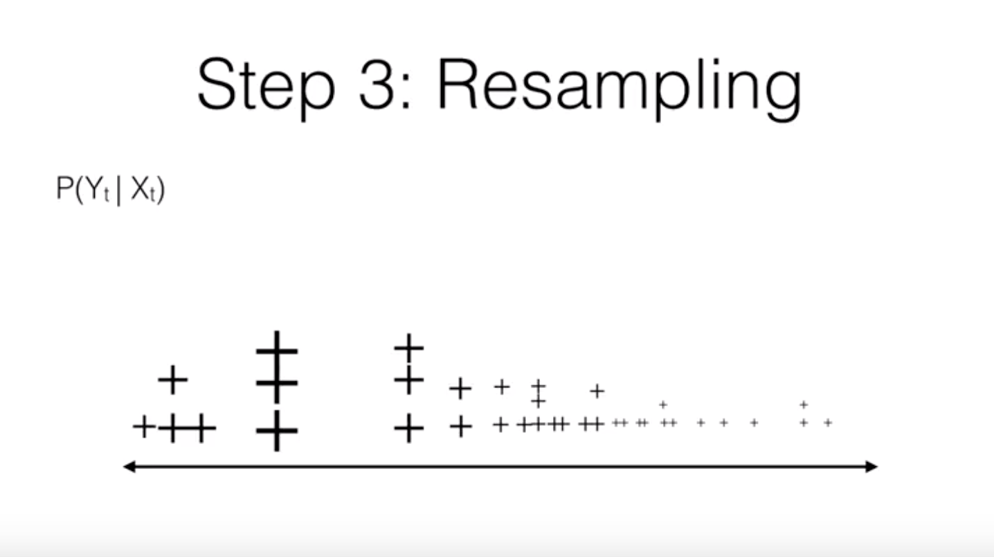
The steps to the algorithm
1. Use n particles to represent distributions over hidden states; create initial values
2. Transition probability: Sample the next state from each particle
3. Calculate the weights and normalize them
4. Resample: generate a new distribution of particles

loop
In pictures

In pictures
In pictures

In pictures
A concrete example

1 sample/s
A concrete example
\phi_n
is a phase angle, given
y_n = \theta_n + v_n
v_n \approx \Nu(0.5^2)
A concrete example

This is the measurement model
A concrete example
This is the measurement model
(it comes from domain knowledge)

A concrete example
This is the process model

w_n \approx \Nu(0, \sigma_{w}^2)
A concrete example
This is state space - now we apply the algorithm

Agenda
- Tools from statistics + Recap
- Particle filters and its components
- An algorithm (In Python)
Modified example based on SciPy
References
Particle Filters
By Hanneli Tavante (hannelita)


