

Hugo Hadfield
Cambridge University PhD student, Signal Processing and Communications Laboratory
Hugo Hadfield, Lai Wei, Joan Lasenby
University Of Cambridge,
Signal Processing and Communications Laboratory
Speaker: Hugo Hadfield
Image source: AEMK Systems
Game engines tick all the boxes
By Hugo Hadfield
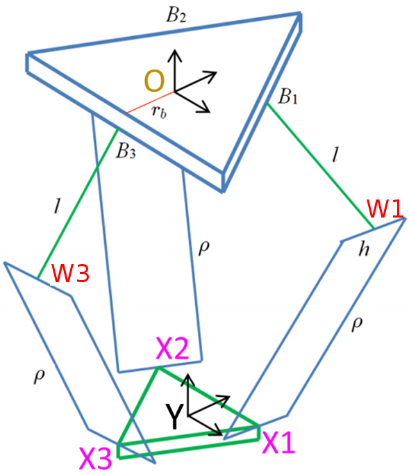
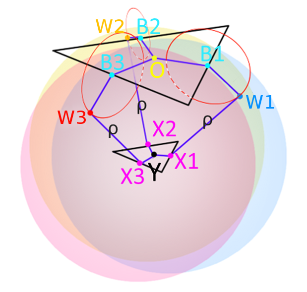
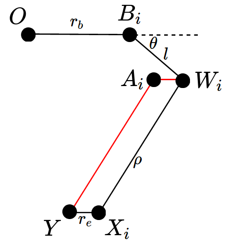
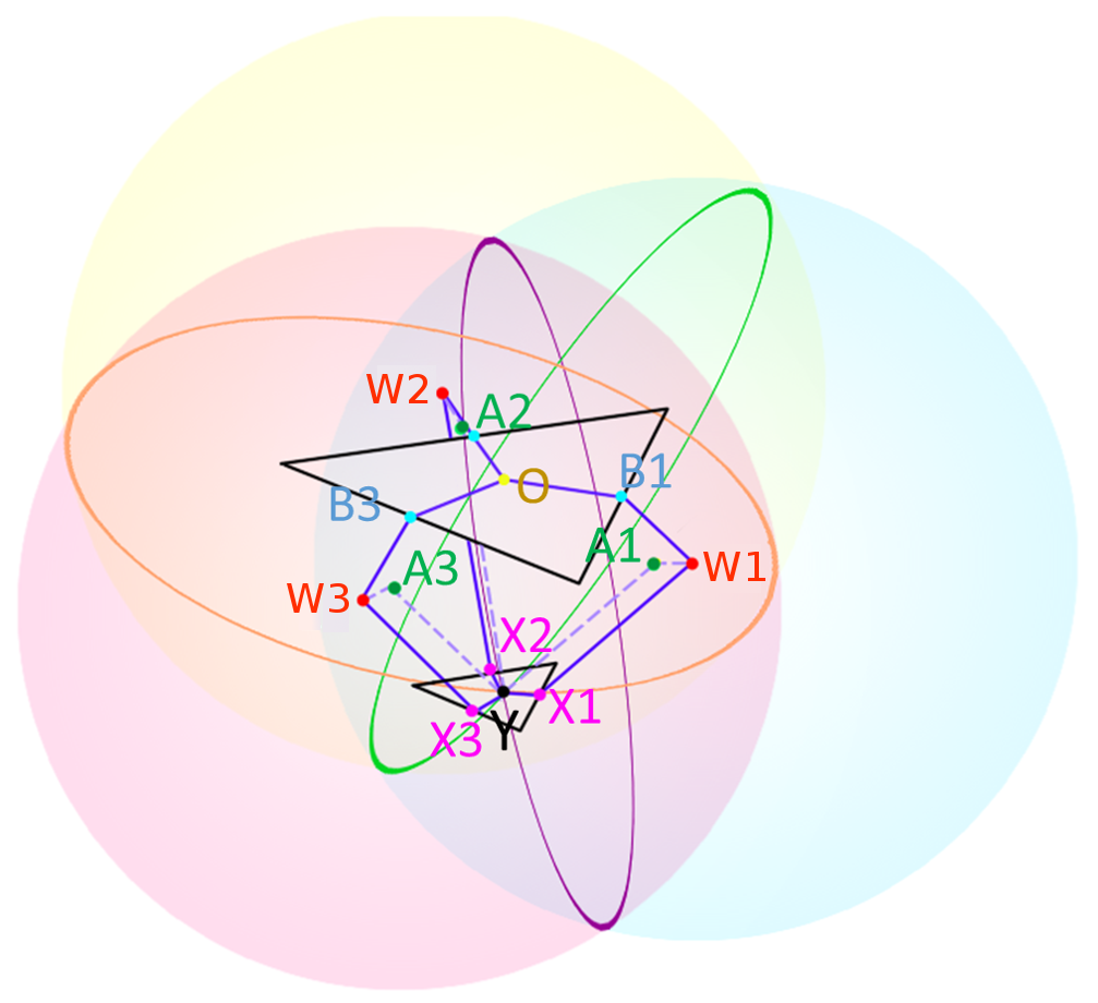
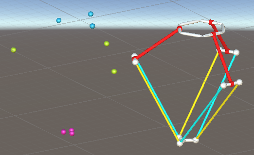
In this presentation we cover the geometry that underlies the forward and inverse kinematic equations of the Delta robot, we present the mathematics in Conformal Geometric Algebra and have interactive demos. Much of this can be found as a part of my PhD thesis here https://hh409.user.srcf.net/thesis/thesis.html


