Probabilistic Voting Model
Lecture 3, Political Economics I
OSIPP, Osaka University
27 October, 2017
Masa Kudamatsu
Did you come up with
a research question
for your term paper?
And is it
original, interesting, and feasible?
For your inspiration #1
Here's the list of policies my undergrad class students have chosen
to write their term paper on why they aren't adopted
For your inspiration #2
Taro Kono's blog (on his early days as a legislator)
For your inspiration #3
Political science books on why DPJ government failed


For your inspiration #4
Questions raised by the last general elections in Japan
Should Prime Minister be allowed to dissolve the parliament?
Do majoritarian elections really help opposition parties?
Why doesn't Japan introduce full proportional representation like in continental Europe?
For your inspiration #5
Instead of voting for one candidate / party,
vote by policy issue
His survey of 75,000 Dutch citizens shows
the correlation between their policy preferences
and the policies proposed by the party they vote
is only 10-20%
Motivations for today
Last week we saw how the citizen-candidate model
relaxes the commitment assumption
The Median Voter Theorem relies on restricting assumptions
This week we'll see how the probabilistic voting model
relaxes the assumption on voters' preference
Single-peaked / Single-crossing for one-dimensional policy
Intermediate preference for multi-dimensional policy
Example: Distribution of Local Public Goods
Demography
Endowment
\(N\) citizens live in several districts, each indexed by \(J\)
Population of district \(J\): \(N^J\)
(\(\sum_J N^J = N\))
Every citizen earns exogenous income \(y\)
(for simplicity)
Example: Distribution of Local Public Goods
Preference of each citizen in district \(J\)
c^J + H(g^J)
Private
consumption
Local
public goods
per capita
where \(H(\cdot)\) is increasing and concave, with \(H(0)=0\)
Government
collects lump sum tax \(\tau\) from every citizen
Government budget constraint
provides per capita local public goods to each district, \(g^J\)
\sum_J N^J g^J = N\tau
Example: Distribution of Local Public Goods (cont.)
District \(J\) citizens' preference over policies
(\Leftarrow \sum_I N^I g^I = N\tau)
W^J(\mathbf{g})=y-\tau+H(g^J)
(\Leftarrow c^J = y - \tau)
=y-\sum_I\frac{N^I}{N}g^I +H(g^J)
Example: Distribution of Local Public Goods (cont.)
District \(J\) citizens' preference over policies
W^J(\mathbf{g})=y-\sum_I\frac{N^I}{N}g^I +H(g^J)
Their ideal policy is given by
H_g(g^J)=1
g^I=0, \forall I \neq J
No "median" policy exists: no equilibrium in Downsian model
Example: Distribution of Local Public Goods (cont.)
g^J
H_g(g^J)
1
Example: Distribution of Local Public Goods (cont.)
Probabilistic voting model does have an equilibrium
as long as citizens' policy preference is continuous and concave
District \(J\) citizens' preference over policies
W^J(\mathbf{g})=y-\sum_I\frac{N^I}{N}g^I +H(g^J)
For the purpose of understanding distortion by politics,
derive the first-best policy:
\max_{\mathbf{g}}\sum_JN^J(c^J+H(g^J))
\text{s.t.} \sum_JN^J(g^J+c^J)=Ny
Sum of utilities
Resource constraint
\max_{\mathbf{g}}[Ny-\sum_JN^Jg^J]+\sum_JN^JH(g^J)
H_g(g^{J,FB})=1, \forall J
Example: Distribution of Local Public Goods (cont.)
First-best given by:
Basic Model
We follow Sections 3.4 & 7.4 of Persson and Tabellini (2000)
Originally proposed by Lindbeck and Weibull (1987)
Players
Each belongs to a group indexed by \(J\)
Two candidates, \(A, B\)
Denote the population share of group \(J\) by \(\alpha^J\)
(\sum_J \alpha^J = 1)
\(N\) citizens, each indexed by \(i\)
Candidates' preference and action
We assume they can commit to this policy
Each candidate's payoff is given by:
Before the election, each announces the policy vector \(\mathbf{q}_A, \mathbf{q}_B\)
Note: we no longer need to stick to one-dimensional policy
So we assume office-seeking politicians
\(R\) if elected (ego-rent)
\(0\) otherwise (normalization)
A way to get round the commitment assumption
Assume there are two political parties, A and B
Each party selects a candidate based on their ideal policy
Remaining issue:
Does the party stick to its candidate after winning the election?
Yes in the U.S.
No in Japan: the ruling party often replaces its leader (ie. Prime Minister) between elections
Citizens' preference
Citizens care about (1) policies and (2) who wins
Citizens' preference
Citizens care about (1) policies and (2) who wins
where \(P\) denotes the winning candidate
Note:
All citizens in the same group have the same preference on policies
W^J(\mathbf{q}_P)
\(W^J(\cdot)\) is a continuous and concave function
\(W^J(\cdot)\) doesn't have to be single-peaked, single-crossing, or intermediate
Citizens' preference
Citizens care about (1) policies and (2) who wins
where \(D_B\) is 1 if B wins and 0 otherwise
Individual ideological bias
\sigma^{iJ}
Population-wide popularity for candidate B
\delta
These two parameters are unknown to candidates
W^J(\mathbf{q}_P)
+ D_B(\sigma^{iJ}+\delta)
Information
Candidates face uncertainty about citizens' preference
W^J(\mathbf{q}_P)
+ D_B(\sigma^{iJ}+\delta)
Known
Unknown
But candidates know the distribution of the unknown parameters
Information (cont.)
Assume the following distributions for population-wide shock:
\big[-\frac{1}{2\psi}, \frac{1}{2\psi}\big]
uniformly distributed over
\delta
Density
\psi
-\frac{1}{2\psi}
\frac{1}{2\psi}
0
\delta
To allow explicit solutions...
Information (cont.)
uniformly distributed over
\sigma^{iJ}
Assume the following distributions for individual bias for B:
\big[-\frac{1}{2\phi^J}, \frac{1}{2\phi^J}\big]
\sigma^{iJ}
Density
\phi^J
-\frac{1}{2\phi^J}
\frac{1}{2\phi^J}
0
Biased for B
Biased for A
To allow explicit solutions...
Information (cont.)
uniformly distributed over
\sigma^{iJ}
\big[-\frac{1}{2\phi^J}, \frac{1}{2\phi^J}\big]
\sigma^{iJ}
Density
\phi^J
-\frac{1}{2\phi^J}
\frac{1}{2\phi^J}
0
For higher \(\phi^J\)
Assume the following distributions for individual bias for B:
To allow explicit solutions...
measures how homogenous group J is
\phi^J
Information (cont.)
These distributions can be generalized
as long as its unimodal and symmetric around the mean
e.g. Normal distribution
Timing of Events
1
2
3
4
Candidates A and B simultaneously announce
their policy platform
\mathbf{q}_A, \mathbf{q}_B
Nature picks individual ideological bias \(\sigma^{iJ}\) and aggregate popularity shocks \(\delta\) for B
Citizens decide which candidate to vote for
The winning candidate implements the announced policy
Analysis
Backward induction
1
2
3
4
Candidates A and B simultaneously announce
their policy platform
Popularity shocks for B, both individual (\(\sigma^{iJ}\)) and aggregate (\(\delta\)), realize
Citizens decide which candidate to vote for
The winning candidate implements the announced policy
\mathbf{q}_A, \mathbf{q}_B
Citizens' optimization
Citizen i of group J votes for A if
W^J(\mathbf{q}_A)>W^J(\mathbf{q}_B)+\sigma^{iJ}+\delta
\sigma^{iJ}<\sigma^J \equiv W^J(\mathbf{q}_A) -
W^J(\mathbf{q}_B)-\delta
or
\sigma^{iJ}
Density
\phi^J
-\frac{1}{2\phi^J}
\frac{1}{2\phi^J}
\sigma^J
Vote for B
Vote for A
\sigma^J \equiv W^J(\mathbf{q}_A) -
W^J(\mathbf{q}_B)-\delta
Citizens' optimization (cont.)
Backward induction
1
2
3
4
Candidates A and B simultaneously announce
their policy platform
Popularity shocks for B, both individual (\(\sigma^{iJ}\)) and aggregate (\(\delta\)), realize
Citizens decide which candidate to vote for
The winning candidate implements the announced policy
\mathbf{q}_A, \mathbf{q}_B
Candidate A's optimization
\max_{\mathbf{q}_A}p_AR + (1-p_A)*0
where the winning probability is given by
p_A=\Pr(\pi_A\geq \frac{1}{2})
A's vote share
How does \(\pi_A\) depend on \(\mathbf{q}_A\)?
\sigma^{iJ}
Density
\phi^J
-\frac{1}{2\phi^J}
\frac{1}{2\phi^J}
\sigma^J
Vote for B
Vote for A
Thus A's vote share among group J citizens is given by
\pi^J_A=\phi^J(\sigma^J-(-\frac{1}{2\phi^J}))
Candidate A's vote share among group J citizens
= \phi^J\sigma^J+\frac{1}{2}
Candidate A's vote share among all citizens
\pi_A=\sum_J \alpha^J\pi^J_A
=\sum_J \alpha^J(\phi^J\sigma^J+\frac{1}{2})
(Remember \(\alpha^J\) denotes group J's population share)
where
\sigma^J \equiv W^J(\mathbf{q}_A) -
W^J(\mathbf{q}_B) -\delta
Unlike in the Downsian model,
here the vote share is a continuous function of policies
thanks to stochastic \(\sigma^{iJ}\)
=\frac{1}{2}+\sum_J \alpha^J\phi^J\sigma^J
Candidate A's vote share among all citizens
\pi_A=\sum_J \alpha^J\pi^J_A
where
\sigma^J \equiv W^J(\mathbf{q}_A) -
W^J(\mathbf{q}_B) -\delta
But candidates maximize the winning probability, not the vote share
If \(\delta\) is known, \(\Pr(\pi_A\geq 1/2)\) is not continuous w.r.t. \(\mathbf{q}_A\)
=\frac{1}{2}+\sum_J \alpha^J\phi^J\sigma^J
Candidate A's vote share among all citizens
\pi_A=\sum_J \alpha^J\pi^J_A
where
\sigma^J \equiv W^J(\mathbf{q}_A) -
W^J(\mathbf{q}_B) -\delta
Random variable when candidates choose their policy
Make the winning probability a continuous function of policies
=\frac{1}{2}+\sum_J \alpha^J\phi^J\sigma^J
Candidate A's winning probability
Rearranging terms...
=\frac{1}{2}+\sum_J\alpha^J\phi^J(W^J(g_A)-W^J(g_B)-\delta)
=\frac{1}{2}+\sum_J\alpha^J\phi^J(W^J(g_A)-W^J(g_B))
Now we want to know the probability that \(\pi_A\geq1/2\)
\pi_A=\frac{1}{2}+\sum_J \alpha^J\phi^J\sigma^J
-\delta\sum_J\alpha^J\phi^J
Candidate A's winning probability
Rearranging terms...
=\frac{1}{2}+\sum_J\alpha^J\phi^J(W^J(g_A)-W^J(g_B)-\delta)
=\frac{1}{2}+\sum_J\alpha^J\phi^J(W^J(g_A)-W^J(g_B))
-\delta\sum_J\alpha^J\phi^J
\pi_A=\frac{1}{2}+\sum_J \alpha^J\phi^J\sigma^J
That is, the probability that these terms are larger than zero
Candidate A's winning probability
\sum_J\alpha^J\phi^J(W^J(g_A)-W^J(g_B))
\geq\delta\sum_J\alpha^J\phi^J
That is, the probability that this inequality holds
Candidate A wins if
\pi_A\geq \frac{1}{2}
or
\sum_J\alpha^J\phi^J(W^J(g_A)-W^J(g_B))\geq \delta\sum_J\alpha^J\phi^J
or
\delta \leq \frac{1}{\phi}\sum_J\alpha^J\phi^J(W^J(g_A)-W^J(g_B))
where
\phi\equiv\sum_J\alpha^J\phi^J
(average homogeneity)
Candidate A's winning probability (cont.)
Candidate A's winning probability
Candidate A wins if
Now since
\delta
is uniformly distributed within
\big[-\frac{1}{2\psi}, \frac{1}{2\psi}\big]
we can obtain the probability that
\pi_A\geq \frac{1}{2}
\delta \leq \frac{1}{\phi}\sum_J\alpha^J\phi^J(W^J(g_A)-W^J(g_B))
\Pr[\delta \leq \frac{1}{\phi}\sum_J\alpha^J\phi^J(W^J(\mathbf{q}_A)-W^J(\mathbf{q}_B))]
\delta
Density
\psi
-\frac{1}{2\psi}
\frac{1}{2\psi}
\frac{1}{\phi}\sum_J\alpha^J\phi^J(W^J(\mathbf{q}_A)-W^J(\mathbf{q}_B))
A wins
=\psi[ \frac{1}{\phi}\sum_J\alpha^J\phi^J(W^J(\mathbf{q}_A)-W^J(\mathbf{q}_B))-(-\frac{1}{2\psi})]
Candidate A's winning probability (cont.)
=\frac{1}{2}+\frac{\psi}{\phi}\sum_J\alpha^J\phi^J(W^J(\mathbf{q}_A)-W^J(\mathbf{q}_B))
Candidate A's winning probability (cont.)
\Pr[\delta \leq \frac{1}{\phi}\sum_J\alpha^J\phi^J(W^J(\mathbf{q}_A)-W^J(\mathbf{q}_B))]
=\psi[ \frac{1}{\phi}\sum_J\alpha^J\phi^J(W^J(\mathbf{q}_A)-W^J(\mathbf{q}_B))-(-\frac{1}{2\psi})]
Note: The winning probability is a continuous function of the policy
cf. This is not the case for the Downsian model
\Pr[\pi_B\geq\frac{1}{2}] = (1-\Pr[\pi_A\geq\frac{1}{2}])
=\frac{1}{2}+\frac{\psi}{\phi}\sum_J\alpha^J\phi^J(W^J(\mathbf{q}_B)-W^J(\mathbf{q}_A))
\Pr[\pi_A\geq\frac{1}{2}]=\frac{1}{2}+\frac{\psi}{\phi}\sum_J\alpha^J\phi^J(W^J(\mathbf{q}_A)-W^J(\mathbf{q}_B))
Candidate A's winning probability
Candidate B's winning probability
Both candidates' objective is
concave in their own action (i.e. policy)
continuous in the other candidate's action
A Nash equilibrium exists
(see e.g. Section 1.3.3 of Fudenberg and Tirole 1991)
\Pr[\pi_B\geq\frac{1}{2}] = (1-\Pr[\pi_A\geq\frac{1}{2}])
Both candidates solve the same maximization problem
In the equilibrium, both candidates propose the same policy
\Pr[\pi_A\geq\frac{1}{2}]=\frac{1}{2}+\frac{\psi}{\phi}\sum_J\alpha^J\phi^J(W^J(\mathbf{q}_A)-W^J(\mathbf{q}_B))
Candidate A's winning probability
Candidate B's winning probability
=\frac{1}{2}+\frac{\psi}{\phi}\sum_J\alpha^J\phi^J(W^J(\mathbf{q}_B)-W^J(\mathbf{q}_A))
W^J(\mathbf{q}_A)=W^J(\mathbf{q}_B)
\sigma^{iJ}
Density
\phi^J
-\frac{1}{2\phi^J}
\frac{1}{2\phi^J}
\sigma^J
Vote for B
Vote for A
\sigma^J \equiv W^J(\mathbf{q}_A) -
W^J(\mathbf{q}_B)-\delta
In the equilibrium...
=-\delta
Implications
Implications from Probabilistic Voting Model
1
Equilibrium policies
maximize the weighted sum of citizens' payoffs
2
Politicians target swing voters, not loyal voters
3
Median voters are not necessarily decisive
Equilibrium policy maximizes a weighted sum of citizen payoffs
\Pr[\pi_A\geq\frac{1}{2}]
=\frac{1}{2}+\frac{\psi}{\phi}\sum_J\alpha^J\phi^J(W^J(g_A)-W^J(g_B))
More populous or more homogenous groups
are treated better
Macroeconomists often use this result to endogenize policies
e.g. Song et al. (2012 Econometrica) on government debt
Implication 1
Each candidate maximizes the winning probability given by
Group J's weight: \(\alpha^J \phi^J\)
Implication 2: Swing Voter Hypothesis
Swing voters: those not loyal to any candidate/party (無党派層)
In the model, those groups with high \(\phi^J\)
\sigma^{iJ}
\phi^J
0
Implication 2: Swing Voter Hypothesis
Swing voters: those not loyal to any candidate/party (無党派層)
The model predicts
politicians mostly please those groups with high \(\phi^J\)
\sigma^{iJ}
\phi^J
0
We now illustrate the swing voter hypothesis
in the example of distribution of local public goods
that we saw at the beginning of this lecture
See Section 7.4 of Persson and Tabellini (2000) for detail
District \(J\) citizens' preference over policies
W^J(\mathbf{g})=y-\sum_I\frac{N^I}{N}g^I +H(g^J)
Example: Distribution of Local Public Goods (revisited)
g^J
H_g(g^J)
1
First-best policies:
H_g(g^J)=1, \forall J
Distribution of Local Public Goods
Candidate's problem
\max_{\mathbf{g}_A}p_AR
p_A=\frac{1}{2}+\frac{\psi}{\phi}\sum_J\alpha^J\phi^J(W^J(\mathbf{g}_A)-W^J(\mathbf{g}_B))
where
\alpha^J=\frac{N^J}{N}
That is,
\max_{\mathbf{g}_A}\frac{\psi}{\phi}\sum_J\alpha^J\phi^JW^J(\mathbf{g}_A)
where
W^J(\mathbf{g}_A)=y-\sum_I\alpha^Ig_A^I +H(g_A^J)
Distribution of Local Public Goods (cont.)
Candidate's problem
\max_{\mathbf{g}_A}\frac{\psi}{\phi}\sum_J\alpha^J\phi^J[y-\sum_I\alpha^Ig_A^I +H(g_A^J)]
Distribution of Local Public Goods (cont.)
FOC w.r.t. \(g^J_A\)
\alpha^J\phi^J[H_g(g_A^J)-\alpha^J]=\alpha^J\sum_{I\neq J}\alpha^I\phi^I
Candidate's problem
\max_{\mathbf{g}_A}\frac{\psi}{\phi}\sum_J\alpha^J\phi^J[y-\sum_I\alpha^Ig_A^I +H(g_A^J)]
\phi^JH_g(g_A^J) =\sum_{I}\alpha^I\phi^I
H_g(g_A^J)=\frac{\sum_I\alpha^I\phi^I}{\phi^J}
Or
Or
Distribution of Local Public Goods (cont.)
FOC w.r.t. \(g^J_A\)
\sigma^{iJ}
\phi^J
H_g(g_A^J)-\alpha^J
Switch to vote for A
For district \(J\)
\alpha^J\phi^J[H_g(g_A^J)-\alpha^J]=\alpha^J\sum_{I\neq J}\alpha^I\phi^I
The gain of voters in district \(J\)
Distribution of Local Public Goods (cont.)
FOC w.r.t. \(g^J_A\)
\sigma^{iJ}
\phi^J
\alpha^J
Switch to vote for B
For districts \(I\neq J\)
\alpha^J\phi^J[H_g(g_A^J)-\alpha^J]=\alpha^J\sum_{I\neq J}\alpha^I\phi^I
The loss of voters in districts \(I\neq J\)
Distribution of Local Public Goods (cont.)
FOC w.r.t. \(g^J_A\)
\phi^JH_g(g_A^J) =\sum_{I}\alpha^I\phi^I
H_g(g_A^J)=\frac{\sum_I\alpha^I\phi^I}{\phi^J}
Or
Or
\alpha^J\phi^J[H_g(g_A^J)-\alpha^J]=\alpha^J\sum_{I\neq J}\alpha^I\phi^I
Distribution of Local Public Goods
FOC w.r.t. \(g^J_A\)
H_g(g_A^J)=\frac{\sum_I\alpha^I\phi^I}{\phi^J}
For groups with \(\phi^J\) higher than the average (\(\sum_I\alpha^I\phi^I\))
H_g(g_A^{J*})=\frac{\sum_I\alpha^I\phi^I}{\phi^J}<1 = H_g(g^{J,FB})
i.e. Politically more responsive voter groups
receive more than socially optimal
Swing Voter Hypothesis
More generally speaking, politicians target voter groups like
\sigma^{iJ}
\phi^J
0
instead of targeting voter groups like
\sigma^{iJ}
\phi^J
0
See Proposition 1 of Casey (2015) for the formal argument on this
Swing Voter Hypothesis
More generally speaking, politicians target voter groups like
\sigma^{iJ}
\phi^J
0
instead of targeting voter groups like
\sigma^{iJ}
\phi^J
0
We'll see evidence for this hypothesis shortly
Implication 3:
Median voters are not necessarily decisive
See Section 3.4 of Persson and Tabellini (2000) for detail
We illustrate this with a policy example (size of government)
from Lecture 1
Size of government
Preference of citizens in group \(J\)
(1-\tau)y^J+H(g)
Three groups of citizens \(J \in {P, M, R} \)
Group \(J\) citizens earn an exogenous income \( y^J \) with
y^P < y^M < y^R
Each group's population share (\(\alpha^J\)) is less than 1/2
Demography
Endowment
Population is normalized to be 1
Size of government
Government budget constraint
\sum_J \alpha^J\tau y^J=g
Citizen's preference over policy
W^J(g)=(1-\frac{g}{\sum_J\alpha^Jy^J})y^J+H(g)
Each group's ideal policy is given by
H_g(g) = y^J/(\sum_J\alpha^Jy^J)
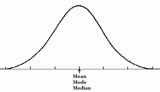
Size of government
Median voter's ideal policy
H_g(g) = y^M/y
will be the equilibrium in the Downsian model
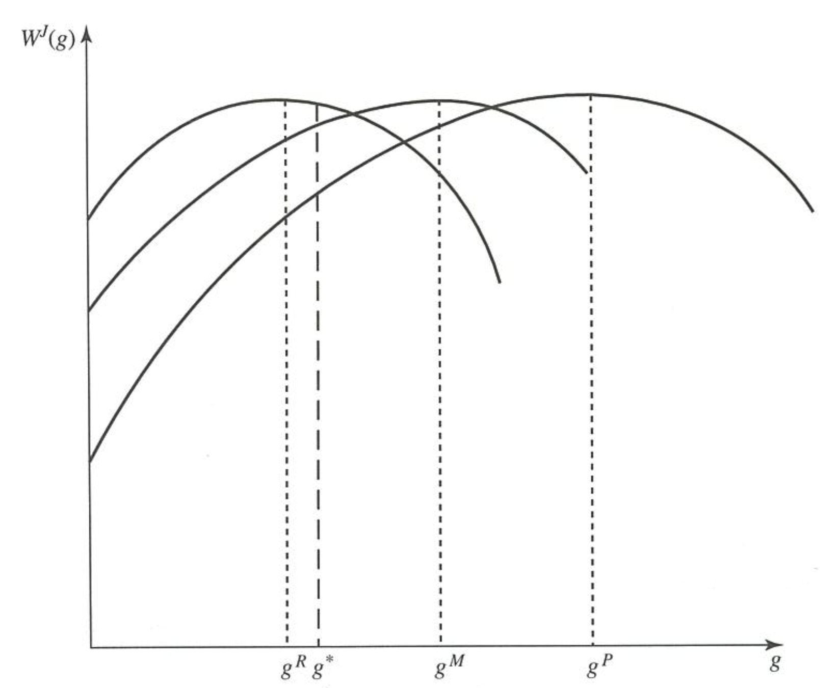
Figure 3.2 of Persson and Tabellini (2000)
Size of government
Median voter's ideal policy
H_g(g) = y^M/y
will be the equilibrium in the Downsian model
Size of government
Candidate's problem
\max_{g_A}p_AR
p_A=\frac{1}{2}+\frac{\psi}{\phi}\sum_J\alpha^J\phi^J(W^J(g_A)-W^J(g_B))
where
That is,
\max_{g_A}\frac{\psi}{\phi}\sum_J\alpha^J\phi^JW^J(g_A)
W^J(g)=(1-\frac{g}{\sum_J\alpha^Jy^J})y^J+H(g)
where
Candidate's problem (cont.)
\max_{g_A}\frac{\psi}{\phi}\sum_J\alpha^J\phi^JW^J(g_A)
=\frac{\psi}{\phi}\sum_J\alpha^J\phi^J[(1-\frac{g_A}{\sum_J\alpha^Jy^J})y^J+H(g_A)]
FOC w.r.t. \(g_A\)
\sum_J\alpha^J\phi^JH_g(g_A)=\frac{1}{\sum_J\alpha^Jy^J}\sum_J\alpha^J\phi^Jy^J
H_g(g_A)=\frac{1}{\sum_J\alpha^Jy^J}(\sum_J\alpha^J\phi^Jy^J/\sum_J\alpha^J\phi^J)
Size of government
FOC w.r.t. \(g_A\)
H_g(g_A)=\frac{1}{\sum_J\alpha^Jy^J}(\sum_J\alpha^J\phi^Jy^J/\sum_J\alpha^J\phi^J)
This term gets closer to \(y^M\)
if \(\phi^M\) is higher than the average
Otherwise,
the equilibrium policy can be far away from the median voter's ideal
Implication 3:
Median voters are not necessarily decisive
Evidence
Empirical challenge
How can we measure "swing voters"?
The literature often uses
winning margin in the previous election
But it's endogenous to distributive policies
The incumbent narrowly won maybe because voters complain about the lack of distributions
(see Larcinese et al. 2013 for a survey and criticism)
(In Lecture 4, we'll see such a model of politics)
And distribution policies are persistent over time
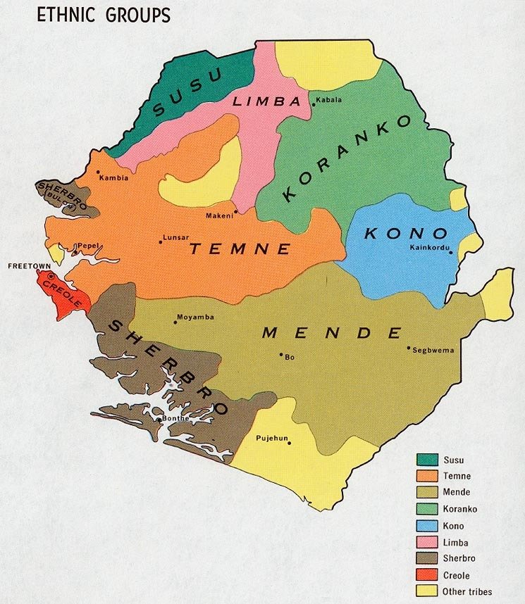
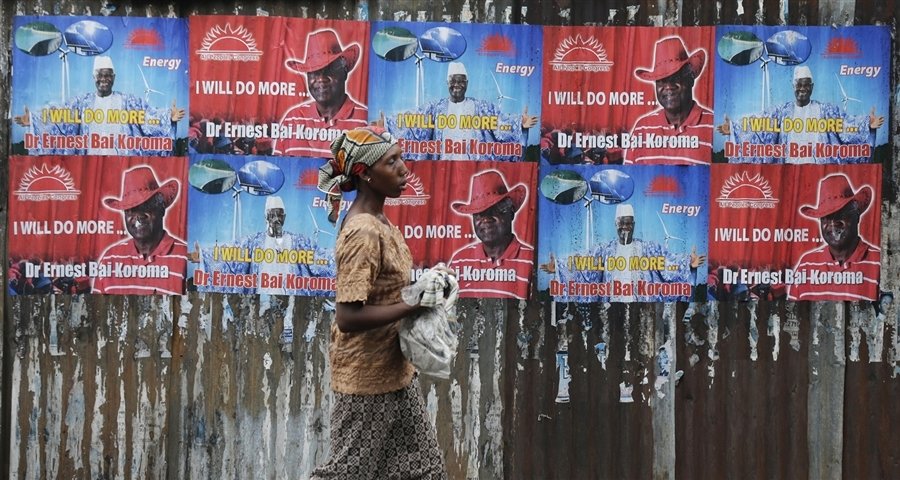
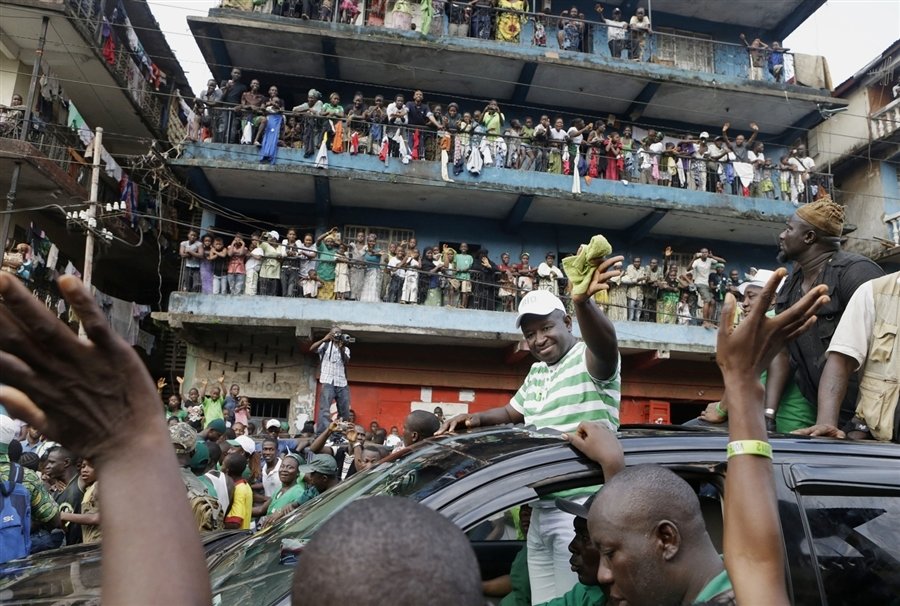
Evidence from Sierra Leone
Casey (2015) overcomes this difficulty
by exploiting ethnic allegiance to political parties in Sierra Leone

Image source: www.bbc.com/news/world-africa-14094194
Ethnic groups in Sierra Leone
Various ethnic groups live in different parts of the country
Political parties in Sierra Leone
SLPP

APC

Two parties have dominated politics since independence in 1961
Measuring ethnic allegiance to parties
Calculate each ethnic group's bias towards APC by:
% of those
who voted for
APC
% of those
who voted for
SLPP
-
Based on nation-wide voting data (for 2007 presidential election)
(not the district-level, which is a response to district-targeting policy)
Data on voting
Exit polls on local council election day in 2008
1117 voters in 59 randomly selected jurisdictions
Household surveys in 2008
6300 citizens in 634 census enumeration areas
(a nationally representative sample)
In both surveys, respondents report which party they voted
in 2007 presidential election
Take the average vote share from both surveys
Table 1 of Casey (2015)
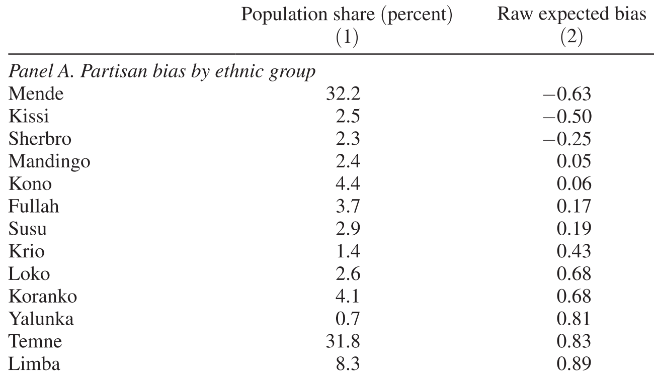
Ethnicity
Population share (%)
Bias to APC
Loyal to APC
Loyal to SLPP
Swing voters
Ethnicity predicts which party to vote
Since ethnicity cannot be changed,
Ethnicity can be used as
a measure of voters' ideology
that's NOT a response to policy !
Measuring swing voter districts
|\alpha_j| = |\sum_e \pi_{ej} \alpha_e|
\pi_{ej}
Population share of ethnic group e in jurisdiction j
\alpha_e
Ethnic group e's bias towards ALC
(based on 2004 census)
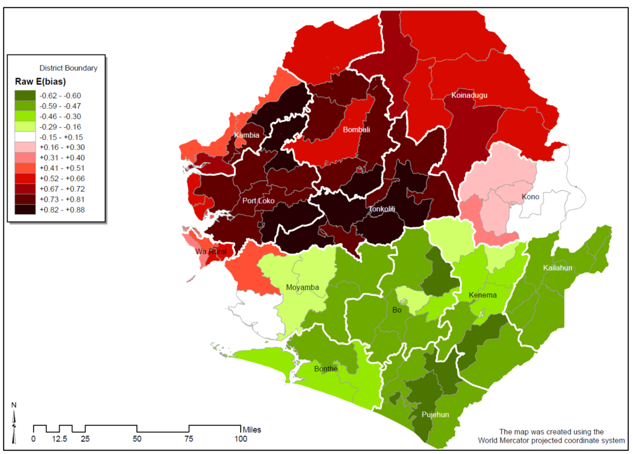
Appendix Figure 1 of Casey (2015)
Light-coloured areas: swing districts
Empirical strategy
Y^i_{jd}=\beta_0 + \beta_1|\alpha_j|+\mathbf{X}'_j\mathbf{\Gamma}+d_d+\varepsilon^i_{jd}
Estimate the following equation by OLS:
Y^i_{jd}
Party i's policy for jurisdiction j in district d
|\alpha_j|
Bias to either of the parties
\mathbf{X}'_j
Vector of jurisdiction j's characteristics
d_d
District fixed effect
Measure of party policy #1
Electoral campaign spendings during the national elections
in 2007
Measure of government policy #2
Local Government Development Grants (LGDG) during 2004-2007
Fiscal transfer from central to local governments
Spent on roads, agriculture, etc.


Check linearity assumption
Y^i_{jd}=\beta_0 + \sum_{k=1}^{34} \beta^k_1 D^k_j+\mathbf{X}'_j\mathbf{\Gamma}+d_d+\varepsilon^i_{jd}
Divide the distribution of \(|\alpha_j|\) into 35 groups with equal frequencies
Let \(D_j^k\) indicate jurisdictions falling into the \(k\)th group
Estimate the following regression by OLS
Then plot the estimated \(\beta_1^k\)'s
Source: Figure 1 of Casey (2015)
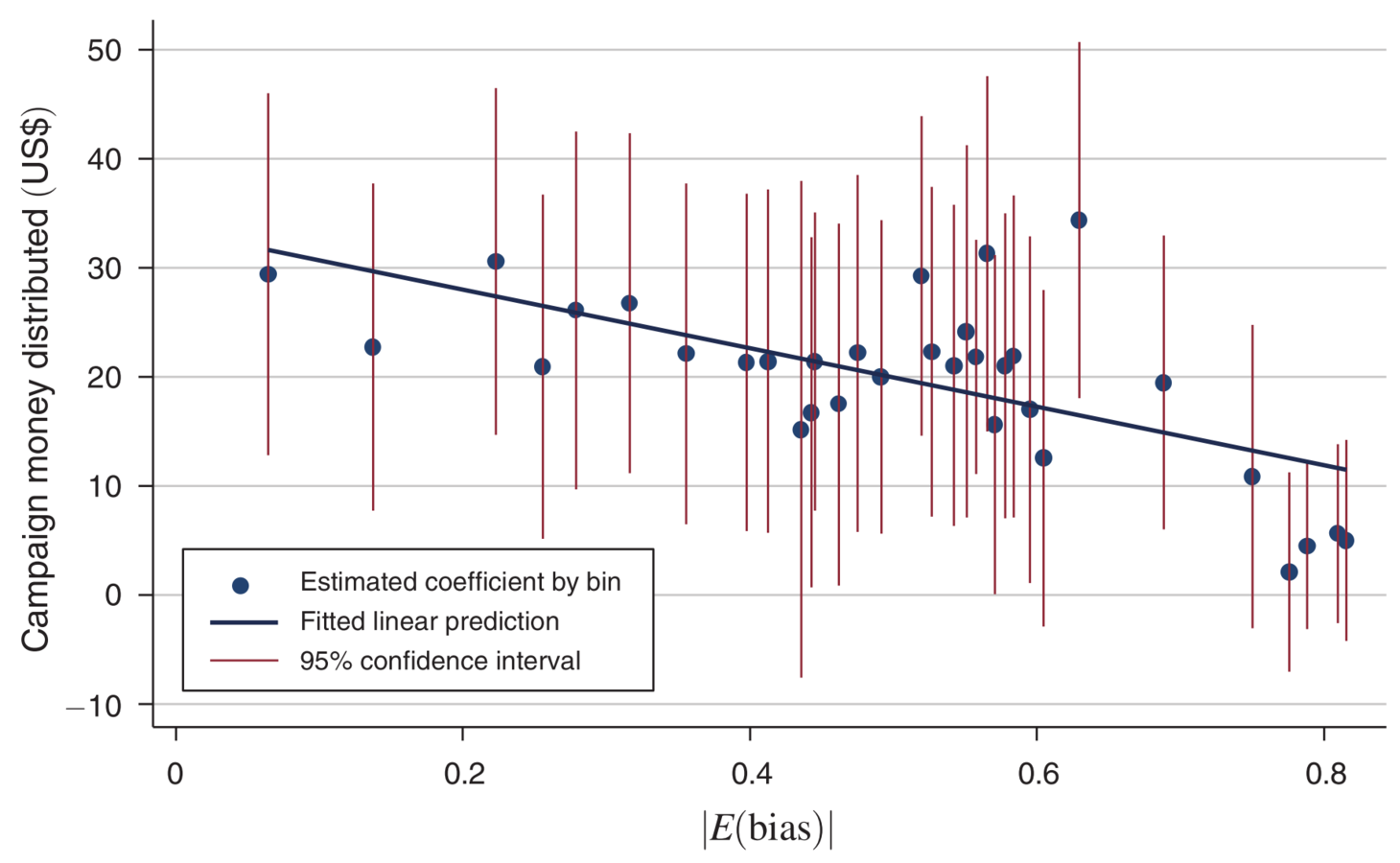
Swing districts attract campaign spendings
Source: Table 2 of Casey (2015)
Swing districts attract various campaign efforts
Similar results for fiscal transfer
If the bias goes down from maximum to minimum
$19,575
(8,757)
reduction in transfer
Source: page 2430 of Casey (2015)
Source: Table 2 of Casey (2015)
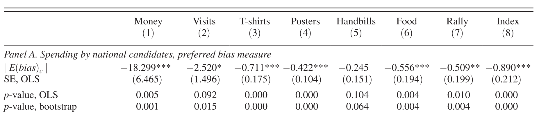
Inference on multiple outcomes
It's time for econometrics...
Inference on multiple outcomes (cont.)
For example, if you have 20 outcomes
the estimated treatment effect
can be statistically significant at the 5% level
for at least 1 outcome by chance
Statistical significance for each outcome is misleading
Inference on multiple outcomes (cont.)
The current standard practice is what Kling et al. (2007) proposed
Transform each outcome into a z-score
z_i^m=\frac{y^m_i - \mu^m}{\sigma^m}
1
Take a simple unweighted average across related outcomes
2
Z_i=\frac{\sum_m z^m_i}{\# m}
3
Estimate the treatment effect on this average z-score
Source: Table 2 of Casey (2015)
Inference on multiple outcomes
Interpretation
Moving from maximum (0) to minimum (1) swing-ness
Campaign efforts go up by 0.89 standard deviation
Applications
Application #1: Incorporate candidate quality
Citizen i of group J votes for A if
W^J(\mathbf{q}_A)>W^J(\mathbf{q}_B)+\sigma^{iJ}+\delta
Casey (2015) interprets \(\delta\) as the relative quality of candidate B
In the basic model, remember:
Its variance gets smaller if citizens are more informed of candidates
Then targeting such citizens is more effective to gain votes
Application #2: Voter intimidation
In the local public good distribution example...
H_g(g_A^J)=\frac{\sum_I\alpha^I\phi^I}{\phi^J}
Swing voters (i.e. high \(\phi^J\)) are "expensive to buy"
In countries like Zimbabwe where incumbent politicians
Consume government revenue
Can intimidate voters from voting
It may pay for incumbents to intimidate swing voters
so they can consume more
Robinson and Torvik (2009) argue...
Other applications for empirical research
Electoral campaign across states by US presidential candidates
Candidate selection by parties across districts in Italy
Impact of radio on New Deal policy in the 1930s US
Other applications for theoretical research
Cause of democratization
Dynamic voting in a macroeconomic model
One more application:
Impact of electoral rules
on the composition of government spending
See also Chapter 8 of Persson and Tabellini (2000)
Model
Players
Three groups of voters
J\in\{1,2,3\}
Each group has a continuum of voters with unit mass
Two political parties
A,B
(So the total population size is 3)
Each lives in its own district
Citizens' preference
Member i of group J
f_A^J+H(g_A)
Transfer to district J
Public
good
f_B^J+H(g_B)+\sigma^{iJ}+\delta
if candidate A wins
if candidate B wins
Citizens' preference (cont.)
Population-wide popularity shock for B
\delta
uniformly distributed between
[-\frac{1}{2\psi},\frac{1}{2\psi}]
Individual ideology for member i of group J
\sigma^{iJ}
uniformly distributed between
[-\frac{1}{2\phi^J}+\bar{\sigma}^J,\frac{1}{2\phi^J}+\bar{\sigma}^J]
with
\bar{\sigma}^1 < \bar{\sigma}^2=0 < \bar{\sigma}^3
and
\phi^2=\max_j[\phi^J]
Graphically...
\sigma^{iJ}
\phi^3
\phi^2
\phi^1
\bar{\sigma}^2(=0)
\bar{\sigma}^1
\bar{\sigma}^3
Policies
f^J
Transfer to district J (e.g. roads, schools, hospitals)
g
Public good (e.g. national defence, social protection)
which satisfy the government budget constraint
\sum_Jf^J+g \leq T
Exogenous govt revenue
Political party's preference & action
p_PR
Each party P maximizes
by committing to a policy vector
\mathbf{q}_P=[ g, \{f^J\}] \geq \mathbf{0}
Timing of Events
1
2
3
4
Parties A and B simultaneously announce
their policy platform
\mathbf{q}_A, \mathbf{q}_B
Nature picks both individual (\(\sigma^{iJ}\)) and aggregate (\(\delta\)) popularity shocks for B
Citizens decide which party to vote for
Electoral rule determines each party's seat share
in legislature
5
The party with the majority of seats forms the government
to implement the announced policy
Electoral rules
Single-district election
(proportional representation)
Multi-district election
(majoritarian)
with sufficiently small \(\bar{\sigma}^1\) and sufficiently large \(\bar{\sigma}^3\)
Denote A's vote share among group J voters by
\pi_{A,J}
Party A wins the majority of seats if
\frac{1}{3}\sum_J\pi_{A,J}\geq\frac{1}{2}
\pi_{A,2}\geq\frac{1}{2}
This is an example of how we can model political institutions
Focus on some features of political institutions
Model them as the rule of the game / the game structure
In this course, we will see more examples:
Term Limit (Lecture 4)
Presidential vs Parliamentary systems (Lecture 5)
Equilibrium
for Single-district Election
District transfer
f^2>0, f^1=f^3=0
Targeting district 2 brings more votes
\sigma^{iJ}
\phi^3
\phi^2
\phi^1
\Delta f^2
\Delta f^3
\Delta f^1
Public good
\sum_J\phi^JH_g(g^*)=\phi^2
\sigma^{iJ}
\phi^3
\phi^2
\phi^1
H_g(g)\Delta g
H_g(g)\Delta g
H_g(g)\Delta g
Vote gains by \(\Delta g\)
Public good
\sum_J\phi^JH_g(g^*)=\phi^2
\sigma^{iJ}
\phi^3
\phi^2
\phi^1
\Delta f^2(=\Delta g)
Vote loss by \(\Delta g\)
Public good in the equilibrium
H_g(g^*)=\phi^2 / \sum_J\phi^J
\sigma^{iJ}
\phi^3
\phi^2
\phi^1
H_g(g)\Delta g
H_g(g)\Delta g
H_g(g)\Delta g
\Delta f^2(=\Delta g)
Equilibrium
for Multiple-district Election
Only district 2 can be swung
\sigma^{iJ}
\phi^3
\phi^2
\phi^1
\sigma^2
\sigma^1
\sigma^3
District transfer
f^2>0, f^1=f^3=0
For districts 1 and 3, the electoral result does not depend on f
Public good
\phi^2H_g(g^*)=\phi^2
\sigma^{iJ}
\phi^3
\phi^2
\phi^1
H_g(g)\Delta g
Vote gain by \(\Delta g\)
Public good
\phi^2H_g(g^*)=\phi^2
\sigma^{iJ}
\phi^3
\phi^2
\phi^1
Vote loss by \(\Delta g\)
\Delta g=\Delta f^2
Public good in the equilibrium
H_g(g^*)=1
\sigma^{iJ}
\phi^3
\phi^2
\phi^1
\Delta g=\Delta f^2
H_g(g)\Delta g
Comparison of
the two electoral rules
Public good provision
Multi-district majoritarian elections
H_g(g^*)=1
Single-district (proportional representation) elections
H_g(g^*)=\phi^2 / \sum_J\phi^J
<1
Equilibrium policy
g^*
smaller in multi-district elections
Other theoretical models
(Lizzeri and Persico 2001, Milesi-Ferretti et al. 2002)
derive similar predictions:
Composition of government expenditure is tilted to
group specific transfers
under
majoritarian elections
public good / universal welfare
under
proportional representation
Impact of electoral rules
on the size of government spending
Austen-Smith (2000) and Milesi-Ferretti et al. (2002) predict
Majoritarian elections lead to a smaller government
Evidence
Causal evidence?
Hard to prove causality running from electoral rules to policies
Electoral rules rarely change
Thus impossible to separate the impact of electoral rules
from that of country characteristics
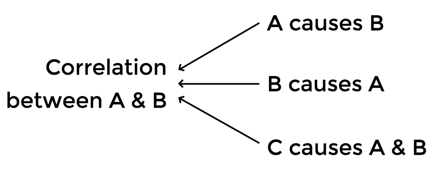
Causal evidence?
We can only check
if correlation is consistent with the theoretical prediction
See also Persson and Tabellini (2003) and Acemoglu (2005)
Run cross-country regressions of fiscal policies on electoral rule
y_i = \beta S_i+\mathbf{Z}_i\mathbf{\Gamma}+\varepsilon_i
\mathbf{Z}_i
Per capita GDP
Trade openness
Population
% of those aged 16-54
% of those aged over 65
Years of being democracy
Quality of democracy (Freedom House Index)
Dummy for presidential system
Dummy for federal states
Dummy for OECD countries
Dummies for continents
Dummies for legal origins
Electoral rules around the world in the 1990s
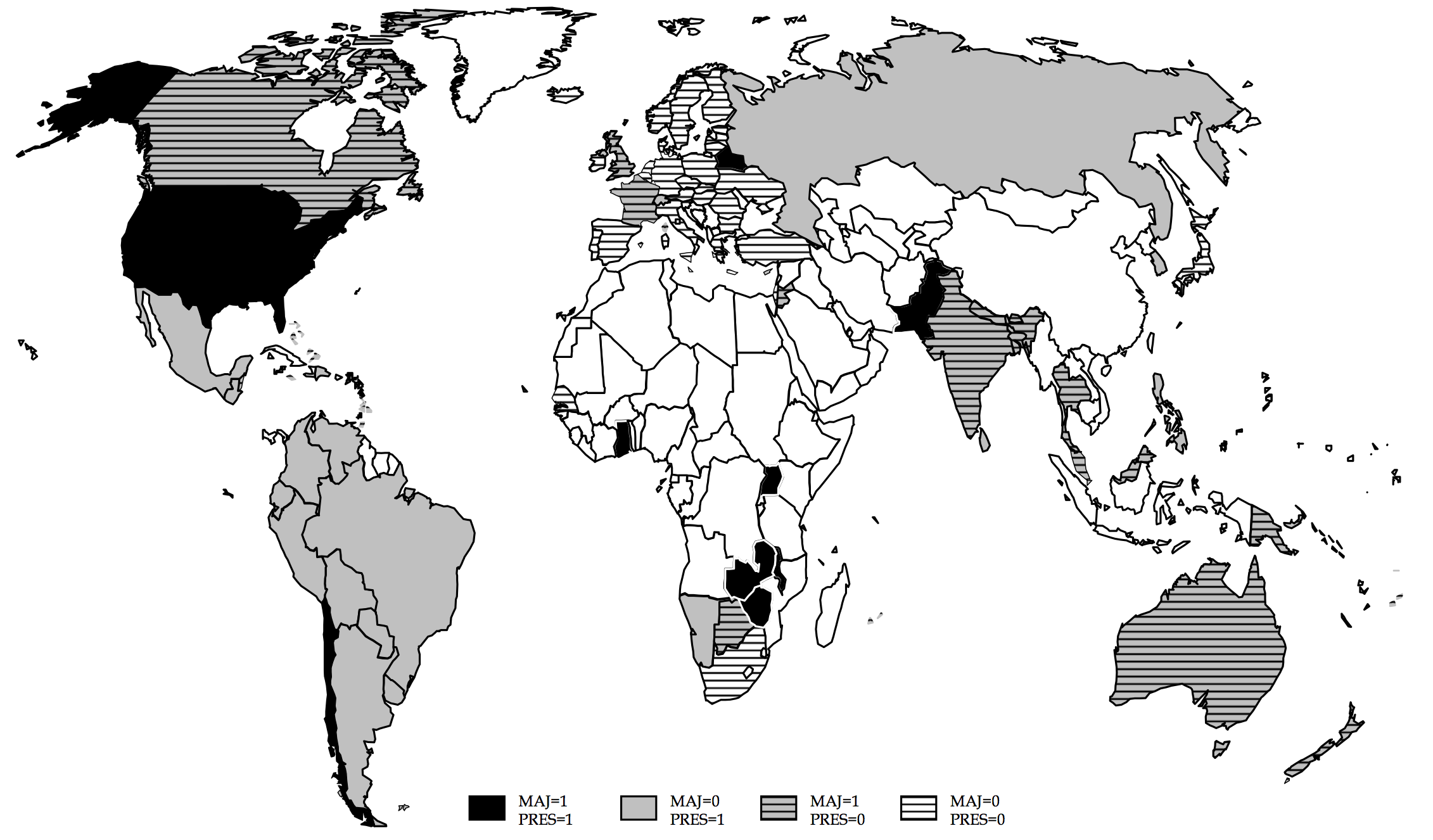
Majoritarian
Proportional Representation
Not democratic
(S_i=1)
(S_i=0)
(excluded from the sample)
Unconditional mean comparison
| Fiscal policy (as % of GDP) |
Central govt expenditure | Social protection |
| Majoritarian | 25.6% (8.2) |
4.7% (5.4) |
| Proportional representation | 30.8% (11.3) |
10.1% (6.6) |
| p-value for two-sample t-test |
Source: Table 1 of Persson and Tabellini (2004)
Note: Standard deviation in parentheses
0.03
0.00
OLS estimation results
| Dep. Var. (as % of GDP) |
Central govt expenditure | Central govt revenue | Government deficit | Social protection |
| Majoritarian elections |
-6.32*** (2.11) |
-3.68* (2.15) |
-3.15*** (0.87) |
-2.25* (1.25) |
| # observations | 80 | 76 | 72 | 69 |
Source: Tables 2 and 4 of Persson and Tabellini (2004)
Countries with majoritarian elections
have a smaller size of government
spend less on social protection (pension, unemployment benefits, child allowance, etc.)
Other impacts of electoral rules
Political selection
Elected politicians are more competent
under a single multi-member district
than under a multiple single-member district
Political Economics lecture 3: Probabilistic Voting Model
By Masayuki Kudamatsu


