Political Agency Model
Lecture 4, Political Economics I
OSIPP, Osaka University
10 November, 2017
Masa Kudamatsu
Motivations
Models in the previous lectures
Political Agency Model
Conflicts of interest
among citizens
Conflicts of interest
between citizens & politicians
e.g.
Income redistribution
Division of a pie
e.g.
Corruption
Disaster relief
Theoretically, an extension of the principal-agent model
The principal (citizens) can only replace the agent (politicians)
as an incentive mechanism
Baseline Model
We follow Section 3.3 of Besley (2006) with a slight modification
Originally(?) proposed by Banks and Sundaram (1993)
Players
Citizens as a single player
Incumbent politician & Opposition candidate
Two preference types (\(i \in \{c,d\}\)):
Denote \(\pi\equiv \Pr(i=c)\)
(can be very close to zero)
We abstract from conflicts among citizens
Congruent (same preference as citizens)
Dissonant (have a personal agenda)
Time, Policy, Election
Two periods, \(t \in \{1,2\}\)
Politician in office in period \(t\) implements a policy denoted by \(e_t \in \{0,1\} \)
Can be infinite horizon (see section 3.4.7 of Besley (2006))
\(e_t = 1\) is a good policy (benefiting citizens)
There is an election between the two periods
Citizens' preference
\Delta
if \(e_t = 1\)
0
otherwise
Discount the next period payoff by \(\beta\)
\sum_{t=1}^2 \beta^{t-1} 1(e_t=1)*\Delta
Citizens' present-value payoff
Politicians' preference (1 of 3)
Both types of politicians yield a payoff of
E
if being in office
0
otherwise
\(E\) includes ego-rent and the wage as a politician
And discount the next period payoff by \(\beta\)
Politicians' preference (2 of 3)
The congruent type of politicians yield an additional payoff of
\Delta
if \(e_t = 1\)
0
otherwise
They share the preference with voters
i.e.
Politicians' preference (3 of 3)
The dissonant type of politicians yield an additional payoff of
0
if \(e_t = 1\)
r_t
otherwise
They have a conflict of interest with voters
where \(r_t \sim G(\cdot)\) with the mean \(\mu\) and the support \([0, R]\)
Examples of \(r_t\)
Private agenda
Capture by special interest or constituency
Disutility from implementing good policy (or incompetence)
i.e.
Information
Voters do not observe
the type of politicians (both incumbent and opposition)
the rent for dissonant politician \(r_t\)
This is a world where politicians know better
Timing of Events (1 of 3)
Period 1
1
Nature picks:
The incumbent politician observes these while voters do not
the type of the incumbent politician \(i \in \{c,d\} \)
the rent for dissonant politician \(r_1\)
2
The incumbent politician chooses policy \(e_1 \in \{0,1\}\)
Period 1 payoffs realize for the incumbent and voters
Timing of Events (2 of 3)
Election
3
Voters decide whether to re-elect the incumbent
But voters do not observe it
4
Nature picks the type of opposition candidate
Timing of Events (3 of 3)
5
The winning politician chooses policy \(e_2 \in \{0,1\}\)
Period 2
Period 2 payoffs realize and the game ends.
6
Nature picks:
the rent for dissonant politician \(r_2\)
Analysis
Equilibrium concept
The model is a dynamic game with incomplete information
i=c
i=d
e_1=1
e_1=1
e_1=0
e_1=0
Nature
Incumbent
Voters
Re-elect
Kick out
Re-elect
Kick out
Re-elect
Kick out
Re-elect
Kick out
Equilibrium concept
Use the Perfect Bayesian Equilibrium
(cf. Section 15.2 of Tadelis 2013)
Politicians behave optimally given the voters' re-election rule
Voters use Bayes rule to update their belief on politician type
The model is a dynamic game with incomplete information
Denote this optimal behavior as \(e_t(i)\)
Period 2 politician's optimization
Since there is no election afterwards,
the politician in office simply chooses his/her own preferred policy:
e_2(c)=1
e_2(d)=0
Politicians' preference (2 of 3)
The congruent type of politicians yield an additional payoff of
\Delta
if \(e_t = 1\)
0
otherwise
Politicians' preference (3 of 3)
The dissonant type of politicians yield an additional payoff of
0
if \(e_t = 1\)
r_t
otherwise
where \(r_t \sim G(\cdot)\) with the mean \(\mu\) and the support \([0, R]\)
Period 2 politician's optimization
Since there is no election afterwards,
the politician in office simply chooses his/her own preferred policy:
e_2(c)=1
e_2(d)=0
Voters want to elect the congruent politician
Voters' optimization
Consider voters' payoff in period 2
i=c
i=d
e_1=1
e_1=1
e_1=0
e_1=0
Nature
Incumbent
Voters
Re-elect
Kick out
Re-elect
Kick out
Re-elect
Kick out
Re-elect
Kick out
Voters' optimization
Opposition candidate is congruent with probability \(\pi\)
i=c
i=d
e_1=1
e_1=1
e_1=0
e_1=0
Nature
Incumbent
Voters
Re-elect
Kick out
Re-elect
Kick out
Re-elect
Kick out
Re-elect
Kick out
\pi\Delta
\pi\Delta
\pi\Delta
\pi\Delta
Voters' optimization
If congruent incumbent is re-elected
i=c
i=d
e_1=1
e_1=1
e_1=0
e_1=0
Nature
Incumbent
Voters
Re-elect
Kick out
Re-elect
Kick out
Re-elect
Kick out
Re-elect
Kick out
\Delta
\pi\Delta
\pi\Delta
\pi\Delta
\pi\Delta
\Delta
Voters' optimization
i=c
i=d
e_1=1
e_1=1
e_1=0
e_1=0
Nature
Incumbent
Voters
Re-elect
Kick out
Re-elect
Kick out
Re-elect
Kick out
Re-elect
Kick out
\Delta
\pi\Delta
\pi\Delta
\pi\Delta
\pi\Delta
\Delta
If dissonant incumbent is re-elected
0
0
Voters optimization
If re-elect, period 2 payoff is
i=c
i=d
e_1=1
e_1=1
e_1=0
e_1=0
Nature
Incumbent
Voters
Re-elect
Kick out
Re-elect
Kick out
Re-elect
Kick out
Re-elect
Kick out
\Delta
\pi\Delta
\pi\Delta
\pi\Delta
\pi\Delta
\Delta
\Pr(i=c | e_1) \Delta
0
0
Voters optimization
If kick out, period 2 payoff is
i=c
i=d
e_1=1
e_1=1
e_1=0
e_1=0
Nature
Incumbent
Voters
Re-elect
Kick out
Re-elect
Kick out
Re-elect
Kick out
Re-elect
Kick out
\Delta
\pi\Delta
\pi\Delta
\pi\Delta
\pi\Delta
\Delta
\pi\Delta
0
0
Voters optimization
It's optimal to re-elect if
i=c
i=d
e_1=1
e_1=1
e_1=0
e_1=0
Nature
Incumbent
Voters
Re-elect
Kick out
Re-elect
Kick out
Re-elect
Kick out
Re-elect
Kick out
\Delta
\pi\Delta
\pi\Delta
\pi\Delta
\pi\Delta
\Delta
\Pr(i=c | e_1)\geq\pi\Delta
0
0
Voters optimization
Voters derive
i=c
i=d
e_1=1
e_1=1
e_1=0
e_1=0
Nature
Incumbent
Voters
Re-elect
Kick out
Re-elect
Kick out
Re-elect
Kick out
Re-elect
Kick out
\Pr(i=c | e_1)
\Delta
\pi\Delta
\pi\Delta
\pi\Delta
\pi\Delta
\Delta
0
0
from incumbent's optimization
Ex post probability of congruent incumbent
\Pr(i=c | e_1=1)
= \frac{\Pr(e_1=1|i=c)\Pr(i=c)}{\Pr(e_1=1)}
(by Bayes' Theorem)
Ex post probability of congruent incumbent
\Pr(i=c | e_1=1)
=\frac{\Pr(e_1=1|i=c)\pi}{\Pr(e_1=1)}
= \frac{\Pr(e_1=1|i=c)\Pr(i=c)}{\Pr(e_1=1)}
(By assumption of \(\Pr(i=c) = \pi \) )
Ex post probability of congruent incumbent
\Pr(i=c | e_1=1)
=\frac{\Pr(e_1=1|i=c)\pi}{\Pr(e_1=1)}
=\frac{\Pr(e_1=1|i=c)\pi}{\pi\Pr(e_1=1|i=c)+(1-\pi)\Pr(e_1=1|i=d)}
= \frac{\Pr(e_1=1|i=c)\Pr(i=c)}{\Pr(e_1=1)}
Ex post probability of congruent incumbent
\Pr(i=c | e_1=1)
=\frac{\Pr(e_1=1|i=c)\pi}{\Pr(e_1=1)}
=\frac{\Pr(e_1=1|i=c)\pi}{\pi\Pr(e_1=1|i=c)+(1-\pi)\Pr(e_1=1|i=d)}
= \frac{\Pr(e_1=1|i=c)\Pr(i=c)}{\Pr(e_1=1)}
Congruent incumbent's optimal behavior
Bayes' rule
\Pr(i=c | e_1=1)
=\frac{\Pr(e_1=1|i=c)\pi}{\Pr(e_1=1)}
=\frac{\Pr(e_1=1|i=c)\pi}{\pi\Pr(e_1=1|i=c)+(1-\pi)\Pr(e_1=1|i=d)}
= \frac{\Pr(e_1=1|i=c)\Pr(i=c)}{\Pr(e_1=1)}
Incongruent incumbent's optimal behavior
Guess and verify
Now we assume it's optimal for voters to
Re-elect the incumbent if and only if \(e_1=1\)
Then derive the optimal policy choice for the incumbent
Finally, given this optimal incumbent's behavior, prove that
Re-elect the incumbent if and only if \(e_1=1\)
is indeed optimal for voters
Period 1 congruent incumbent's optimization
When voters re-elect the incumbent if and only if \(e_1=1\)
So it's optimal for the congruent incumbent to pick \(e_1=1\)
E + \Delta + \beta(E + \Delta) > E
Payoff from \(e_1=1\)
Payoff from \(e_1=0\)
\Pr(e_1=1|i=c)=1
Period 1 incongruent incumbent's optimization
the condition for the incongruent incumbent to pick \(e_1=1\):
0 + \beta (E+E(r_2)) > r_1 + 0
Payoff from \(e_1=1\)
Payoff from \(e_1=0\)
When voters re-elect the incumbent if and only if \(e_1=1\)
Politicians' preference (3 of 3)
The dissonant type of politicians yield an additional payoff of
0
if \(e_t = 1\)
r_t
otherwise
where \(r_t \sim G(\cdot)\) with the mean \(\mu\) and the support \([0, R]\)
Period 1 incongruent incumbent's optimization
the condition for the incongruent incumbent to pick \(e_1=1\):
0 + \beta (E+E(r_2)) > r_1 + 0
Payoff from \(e_1=1\)
Payoff from \(e_1=0\)
\Pr(e_1=1|i=d)=G(\beta(E+\mu))
When voters re-elect the incumbent if and only if \(e_1=1\)
(\mu \equiv E(r_2))
Voters' optimization when observing \(e_1=1\)
\Pr(e_1=1|i=d)=G(\beta(E+\mu))
Now we know
\Pr(e_1=1|i=c)=1
Plug these into
\Pr(i=c | e_1=1) =\frac{\Pr(e_1=1|i=c)\pi}{\pi\Pr(e_1=1|i=c)+(1-\pi)\Pr(e_1=1|i=d)}
=\frac{\pi}{\pi+(1-\pi)G(\beta(E+\mu))}
>\pi
as long as \(G(\beta(E+\mu))<1\)
So it's optimal to re-elect the incumbent if \(e_1=1\)
\Pr(e_1=0|i=d)=1-G(\beta(E+\mu))
We now know
\Pr(e_1=0|i=c)=0
Plug these into
\Pr(i=c | e_1=0) =\frac{\Pr(e_1=0|i=c)\pi}{\pi\Pr(e_1=0|i=c)+(1-\pi)\Pr(e_1=0|i=d)}
=0
<\pi
So it's optimal to kick out incumbent if \(e_1=0\)
Voters' optimization when observing \(e_1=0\)
Guess and verify
Now we assume it's optimal for voters to
Re-elect the incumbent if and only if \(e_1=1\)
Then derive the optimal policy choice for the incumbent
Finally, given this optimal incumbent's behavior, prove that
Re-elect the incumbent if and only if \(e_1=1\)
is indeed optimal for voters
Are there other equilibria? (1 of 2)
What if voters always re-elect or kick out the incumbent?
\(e_1=1, e_2=1\) if congruent
Then the incumbent simply picks the policy they like in both periods
\(e_1=0, e_2=0\) if dissonant
But then by observing \(e_1\) voters know the type of the incumbent
Re-electing the dissonant incumbent is not optimal
(0 < \pi\Delta)
Kicking out the congruent incumbent is not optimal
(\pi\Delta < \Delta)
This is not an equilibrium
Are there other equilibria? (2 of 2)
Do voters re-elect the incumbent if and only if \(e_1=0\)?
If \(E > (1-\beta) \Delta \),
congruent incumbent prefers being re-elected than choosing \(e_1=1\)
In this case, both types then choose \(e_1=0\)
This is a Perfect Bayesian Equilibrium
as long as voters' off-the-equilibrium belief is that
the incumbent is dissonant if \(e_1=1\)
This equilibrium is ruled out by the Intuitive Criterion of Cho and Kreps (1987)
(cf. Section 16.3 of Tadelis (2013))
Proposition
(1) Period 1 policy is given as follows:
otherwise
e_1=1
if the incumbent is congruent
or if the incumbent is dissonant and \(r_1 < \beta(E+\mu)\)
e_1=0
(2) Voters re-elect the incumbent as long as
e_1=1
Implications
The welfare impact of elections
\pi(1+\beta)\Delta
if there is no election
The welfare impact of elections
\pi(1+\beta)\Delta
if period 1 incumbent is congruent
+(1-\pi)G(\beta(E+\mu))\Delta
if period 1 dissonant incumbent is disciplined
+(1-\pi)[1-G(\beta(E+\mu))]\pi\beta\Delta
if period 1 dissonant incumbent is replaced by a congruent opposition
Disciplining effect of election
Screening effect of election
Alternative modelling approaches
Pure moral hazard (no hidden type)
Pioneered by Barro (1973) and Ferejohn (1986)
On the equilibrium path, citizens are indifferent
between the incumbent and the opposition candidate
This equilibrium is not robust
to allowing the heterogeneity among politicians (Fearon 1999)
Career Concern Model
Originally proposed by Holstrom (1999) for employees
Applied to policy-makers by Dewatripont et al. (1999)
The model assumes that policy-makers do not know their own type
Fine if the type is competence
Implausible if the type concerns preference
Evidence
Citizens punish the incumbent
if his/her performance is worse than expectation
Given this behavior of citizens
Incumbent restrains from shirking, being corrupt, etc.
Two predictions from the political agency model
1
2
Over-invoicing
Corruption by Brazilian mayors
1
2
Pay five times more than cost to a road-building firm
and get kickback
e.g.
Diversion of public funds
e.g.
Pocket fiscal transfer from the Ministry of Health
by forging fake receipt for medical equipment purchase
3
Illegal procurement
e.g.
Only one firm satisfies the qualification
to bid for the construction of a stadium
pp. 710-711 of Ferraz and Finan (2008)
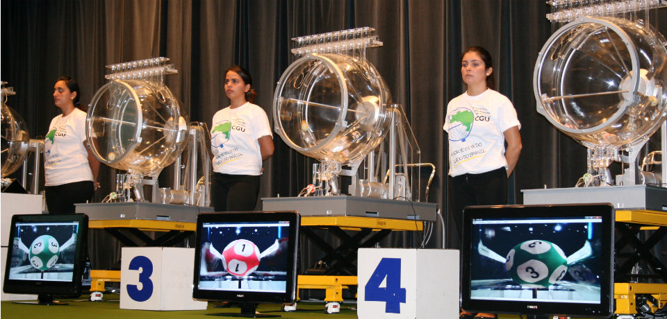
Random auditing of municipal govt expense
Starting from May 2003...
50-60 municipalities per month (out of 5,000+ in total)
randomly chosen for auditing by public lottery
Lottery: witnessed by citiznes, the press, and political parties
Image source: Foreign Policy (2015)
Random auditing of municipal govt expense
Starting from May 2003...
50-60 municipalities per month (out of 5,000+ in total)
randomly chosen for auditing by public lottery
10-15 auditors sent to each chosen municipality
Trained, well-paid, hired by competitive examination
Report is published to the press and on the Internet
Random auditing of municipal govt expense
By the way, the political reasons for randomization were:
Nobody could accuse the auditing agency
of picking their targets through political calculation.
It would discipline mayors even without being investigated
(the auditing agency's budget was limited)
To gauge the nation-wide magnitude of corruption
from the representative sample of municipalities
according to Foreign Policy (2015)
Citizens punish the incumbent
if his/her performance is worse than expectation
Given this behavior of citizens
Incumbent restrains from shirking, being corrupt, etc.
Two predictions from the political agency model
1
2
Tested by Ferraz and Finan (2008)
October 2004
Municipal elections
376 municipalities
audited
300 municipalities
audited
Voters observe
mayor's corruption
before election
Voters don't observe
mayor's corruption
before election
Similar due to random assignment
Difference in
electoral outcomes
Impact of observing
mayor's corruption
=
Research design for 1st prediction
Data
Corruption: # of violations recorded in the audit report
Election outcomes & candidate characteristics
Source: Tribunal Superior Eleitoral
Municipality demographic characteristics
Source: Population census in 2000
Municipality institutional characteristics (e.g. # of radio stations)
Source: Municipality survey in 1999
Available also for those audited after the 2004 elections
Checking the balancedness
Source: Table 1 of Ferraz and Finan (2008)
Only 3 out of 90 variables are significantly different at 5%
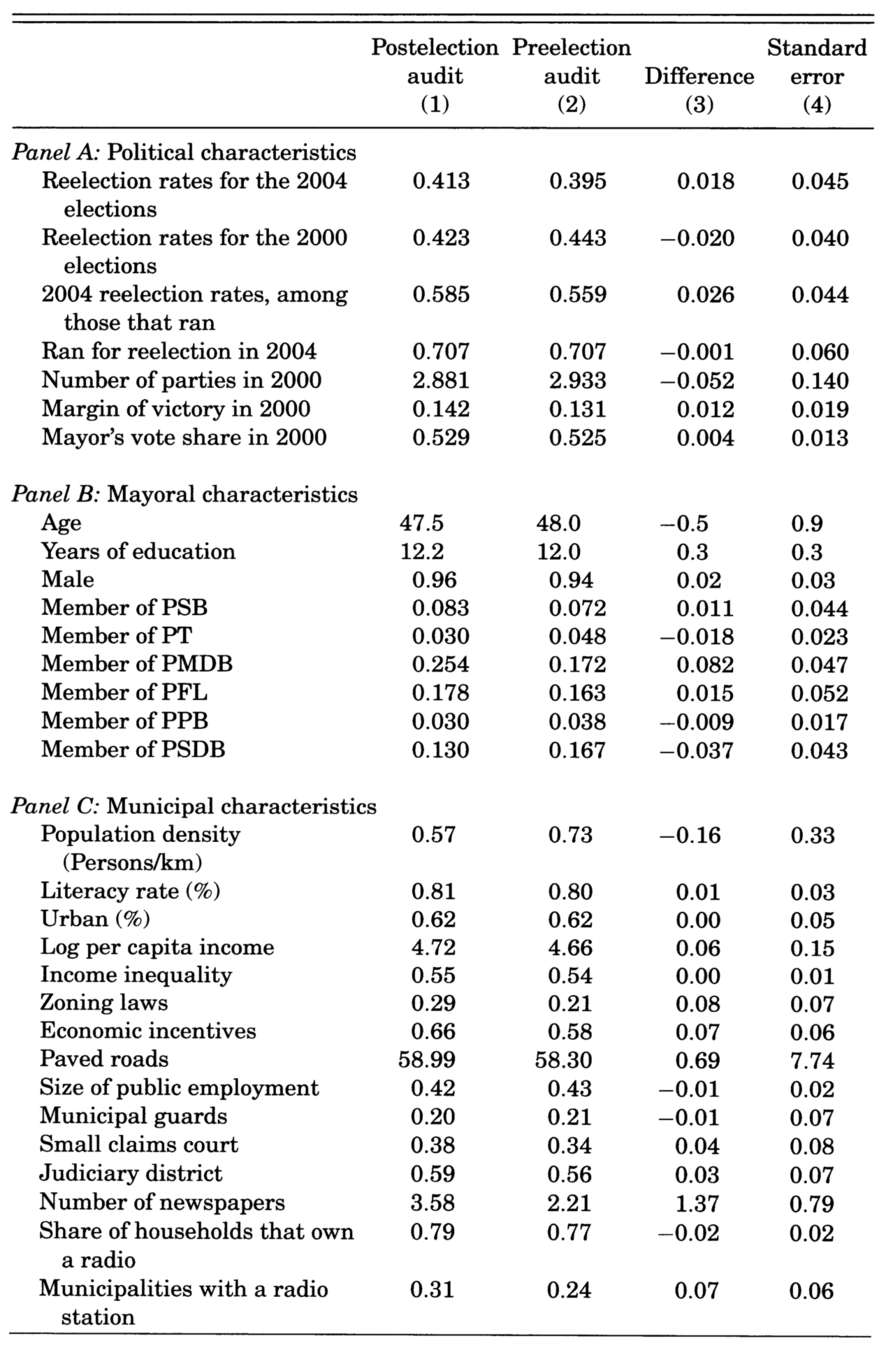
For unbalanced variables...
Standard practice:
Check the robustness to controlling for unbalanced variables
Bruhn and McKenzie (2009) argue
"unbalanced-ness" should refer to economically, not statistically, significant difference
If a covariate is strongly correlated with the outcome,
its large, if insignificant, difference does matter
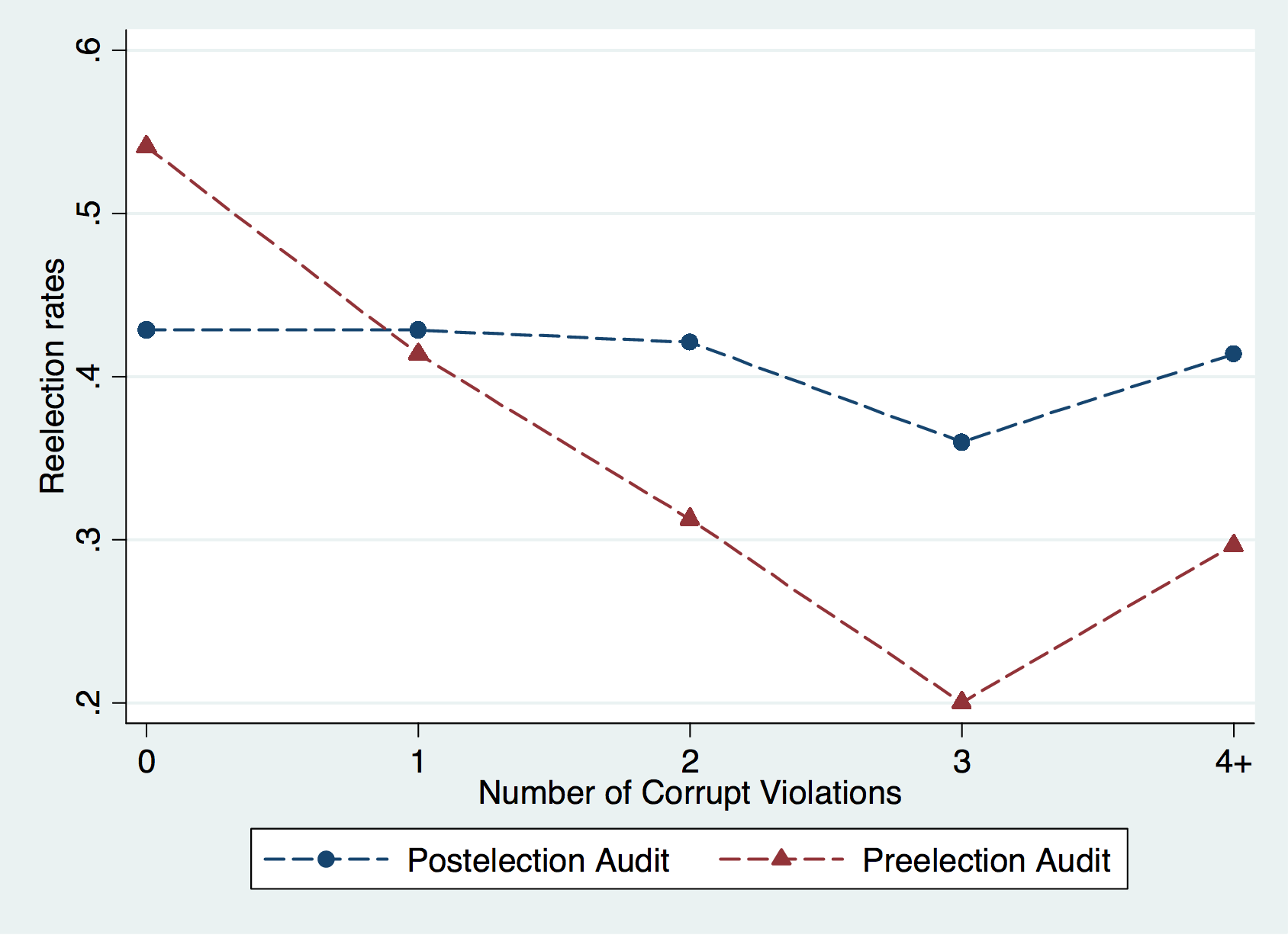
Source: Figure 3 of Ferraz and Finan (2008)
Main Finding
Zero corruption
Re-election
more likely
Source: Figure 3 of Ferraz and Finan (2008)
Finding
2+ violations
Re-election
less likely
Source: Figure 3 of Ferraz and Finan (2008)
Finding
1 violation
Re-election rate
does not change
Citizens expect opposition's violation to be 1
Empirical specification
E_{ms} = \sum_{i} \beta^i_0 C^i_{ms} + \beta_1 A_{ms} + \sum_i \beta^i_2 C^i_{ms}A_{ms}
Indicator of mayor's re-election in municipality \(m\) in state \(s\)
Indicator of being audited before the election
Municipality / Mayor characteristics
State fixed effect
\(E_{ms}\)
\(A_{ms}\)
\(\mathbf{X}_{ms}\)
\(\nu_s\)
Indicator of \(i\) violations found by audit (\(i=1\) omitted)
\(C^i_{ms}\)
+ \mathbf{X}_{ms}\mathbf{\gamma}+\nu_s+\varepsilon_{ms}
Empirical specification
E_{ms} = \sum_{i} \beta^i_0 C^i_{ms} + \beta_1 A_{ms} + \sum_i \beta^i_2 C^i_{ms}A_{ms}
+ \mathbf{X}_{ms}\mathbf{\gamma}+\nu_s+\varepsilon_{ms}
Impact of audit for municipalities with 1 violation
\(\beta_1\)
Impact of audit for municipalities with \(i\) violation
\(\beta^i_2\)
We should see \(\beta_1=0\), \(\beta^0_2>0\), \(\beta^i_2<0\) for \(i\geq 2\)
Results
Source: Table 3 Column 4 of Ferraz and Finan (2008)
| Pre-election audit | 0.084 [0.104] |
| Pre-election audit x 0 violation |
0.010 [0.156] |
| Pre-election audit x 2 violations |
-0.253* [0.148] |
| Pre-election audit x 3 violations |
-0.321* [0.192] |
| Pre-election audit x 4+ violations |
-0.159 [0.168] |
| # of observations | 373 |
* Significant at 10%
Citizens punish the incumbent
if his/her performance is worse than expectation
Given this behavior of citizens
Incumbent restrains from shirking, being corrupt, etc.
Two predictions from the political agency model
1
2
Tested by Ferraz and Finan (2011)
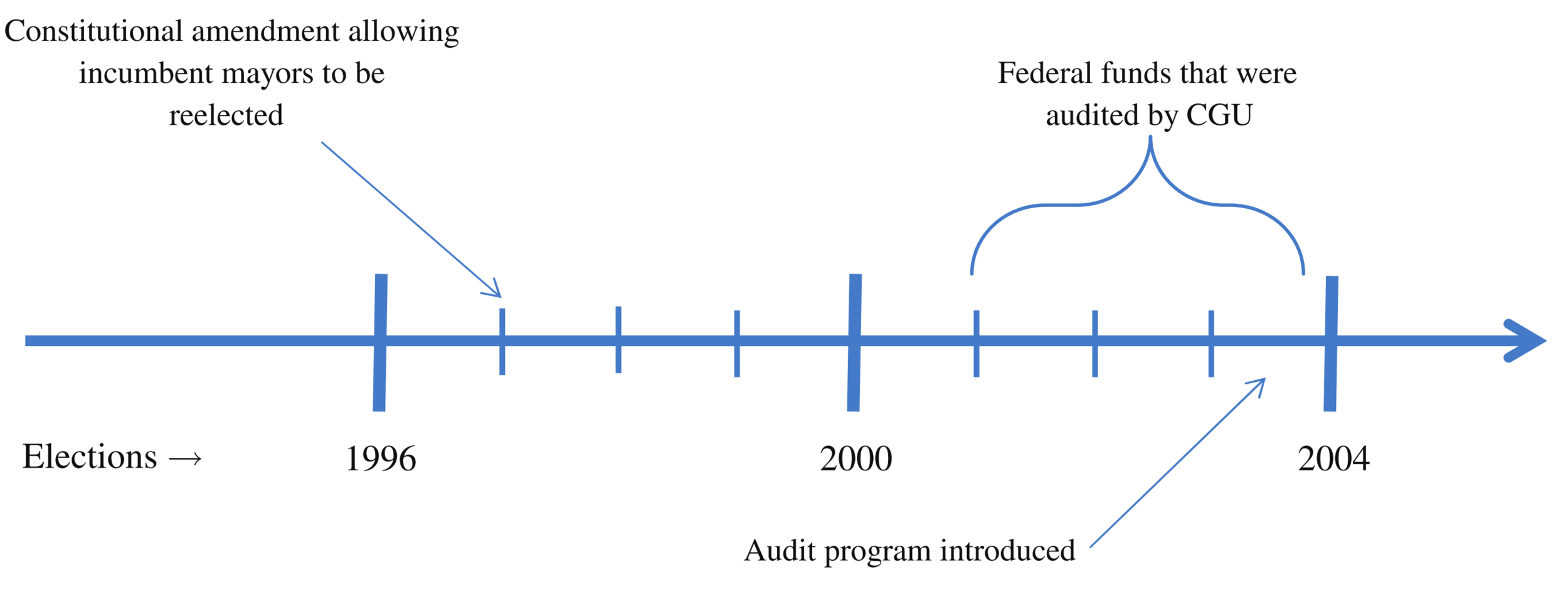
Term limit for Brazilian mayors
Term length = 4 years
Source: Figure 1 of Ferraz and Finan (2011)
Term limit for Brazilian mayors
Source: Figure 1 of Ferraz and Finan (2011)
In 1997, the term limit was extended from one-term to two terms
Term limit for Brazilian mayors
Source: Figure 1 of Ferraz and Finan (2011)
The first mayoral elections since the reform were held in 2000
Research design for 2nd prediction
Compare mayor's corruption during 2001-2004 between
Municipalities where
incumbent barely won
in 2000
& term-limited in 2004
Municipalities where
opposition barely won
in 2000
& can be re-elected in 2004
Source: Figure 1 of Ferraz and Finan (2011)
Research design for 2nd prediction
Compare mayor's corruption during 2001-2004 between
Municipalities where
incumbent barely won
in 2000
& term-limited in 2004
Municipalities where
opposition barely won
in 2000
& can be re-elected in 2004
Similar on average
Difference in corruption = Impact of term limit
Empirical Specification
Regression discontinuity design:
r_i = \beta I_i + f(W_i)+\mathbf{X}_i\mathbf{\Gamma}+\varepsilon_i
Amount of resources related to corruption by mayor \(i\) in office for 2001-2004 (% of total amount of audited resources)
\(r_i\)
\(I_i\)
Indicator of serving the first term (i.e. not term-limited)
\(W_i\)
Vote share margin by the incumbent in the 2000 election
(so \(I_i = 1[W_i< 0]\))
\(\mathbf{X}_i\)
Municipality / Mayor characteristics
Empirical Specification
Regression discontinuity design:
r_i = \beta I_i + f(W_i)+\mathbf{X}_i\mathbf{\Gamma}+\varepsilon_i
Political agency model predicts \(\beta < 0\)
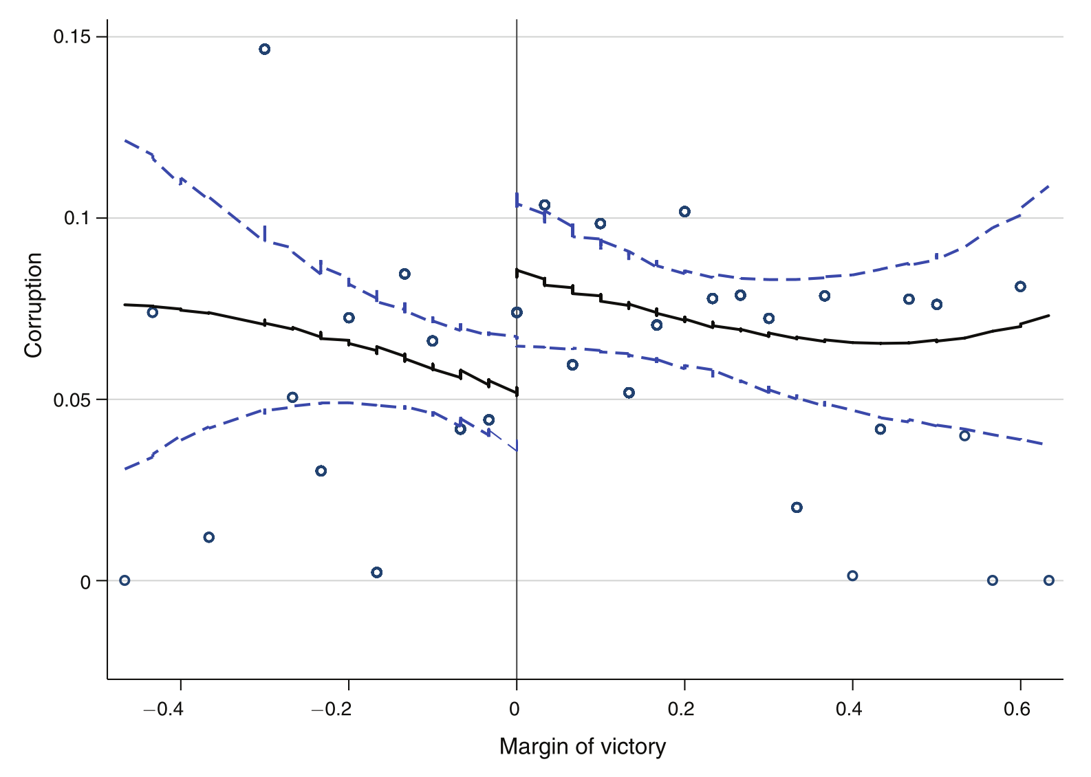
Source: Figure 2 of Ferraz and Finan (2011)
Finding
Term-limited
Results
Source: Table 5 of Ferraz and Finan (2011)

Sample: municipalities where the incumbent ran in 2000
Polynomial functional form
(1) \(f(W_i)=0\)
(2) \(f(W_i)=\alpha W_i\)
(3) \(f(W_i)=\alpha_1 W_i + \alpha_2 W_i^2\)
(4) \(f(W_i)=\alpha_1 W_i + \alpha_2 W_i^2 + \alpha_3 W_i^3\)
Results
Source: Table 5 of Ferraz and Finan (2011)
Sample: municipalities where the incumbent ran in 2000
Polynomial functional form
(5) \(f(W_i)=\alpha W_i + \alpha^I I_i*W_i \)
(6) \( f(W_i)=\alpha_1 W_i + \alpha_2 W_i^2 + \alpha^I_1 I_i*W_i + \alpha^I_2 I_i*W_i^2 \)
(7) \(f(W_i)=\alpha_1 W_i + \alpha_2 W_i^2 + \alpha_3 W_i^3 + \alpha_1^I I_i*W_i + \alpha_2^I I_i*W_i^2 + \alpha_3^I I_i*W_i^3\)
Digression: Polynomial functional form for RDD
Otherwise, use the polynomial of various orders and check if the estimated \(\beta\) is stable across specifications
\(f(W_i)=\alpha W_i + \alpha^I I_i*W_i \)
r_i = \beta I_i + f(W_i)+\mathbf{X}_i\mathbf{\Gamma}+\varepsilon_i
If there are many observations around the cutoff (\(W_i=0\))
Use
Restrict the sample by the method of Calonico et al. (2014)
Known as "local linear regression" (Lee and Lemieux 2010)
Robustness check #1
Source: Table 6 Columns (1) and (5) of Ferraz and Finan (2011)
| Sample | 2nd-term and 1st-term later re-elected |
|
| Mayor in first-term | -0.040*** [0.013] |
|
| # of observations | 313 |
*** Significant at 1%
2nd-term mayors may differ from 1st-term mayors in the ability
(which is why 2nd-term mayors were re-elected)
Drop 1st-term mayors who wouldn't be re-elected in 2004
Robustness check #2
Source: Table 6 Columns (1) and (5) of Ferraz and Finan (2011)
*** Significant at 1%
2nd-term mayors may differ from 1st-term mayors in the experience
(which is why 2nd-term mayors could have learned to be corrupt)
Drop 1st-term mayors who weren't mayor before
| Sample | 2nd-term and 1st-term later re-elected |
2nd-term and 1st-term served as mayor before |
| Mayor in first-term | -0.040*** [0.013] |
-0.038*** [0.014] |
| # of observations | 313 | 287 |
Is the impact economically significant?
Source: Table 2 of Ferraz and Finan (2011)
The estimated impact of not being term-limited is
in the range of -0.03 and -0.04
The average level of corruption: 0.063
Re-election incentive reduces corruption
by around a half
Application
Impact of Term Limits
Term limits in Japan
No term limit for any political offices in Japan
Term limit for LDP President is de facto non-binding
as most presidents resign within 2 years
cf.
Argument against term limits in Japan: "Unconstitutional" (Wikipedia)
"the inalienable right to choose their public officials and to dismiss them"
Article 15
Article 22
Freedom of occupation
Term limits across the world
US: Term limit for President and two-thirds of State Governors
Latin America and Africa
Term limits for presidents were introduced when democratized
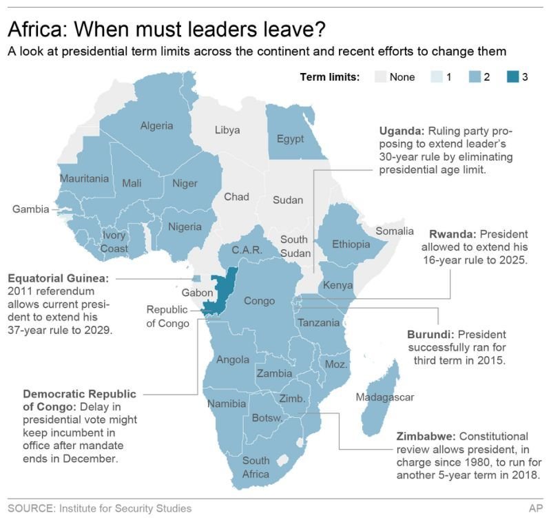
cf. China:
de facto term limit (10 years)
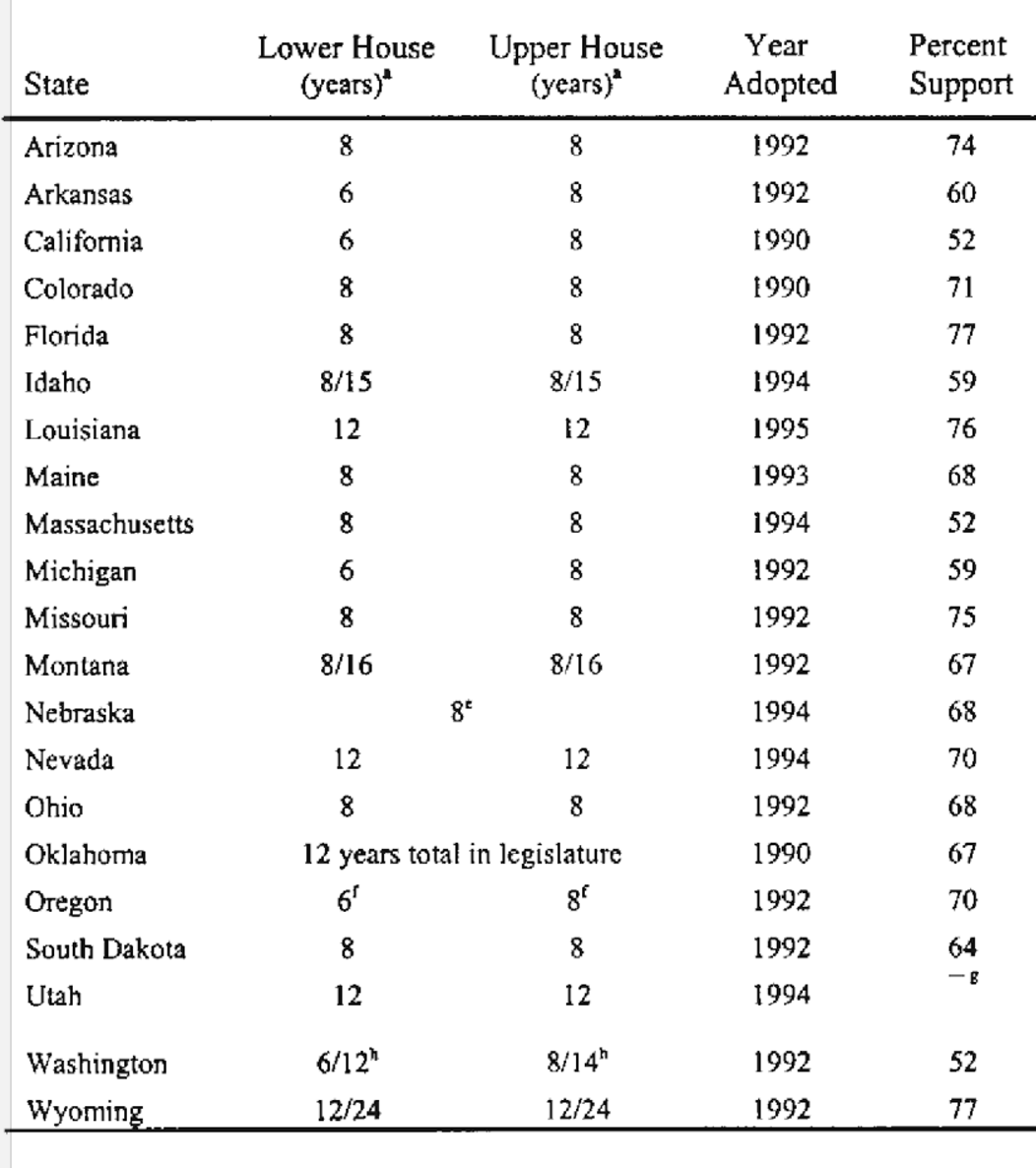
21 US states introduced
term limits for legislators
by referendum in the '90s
Source: Table 1.1 of Carey et al. (2000)
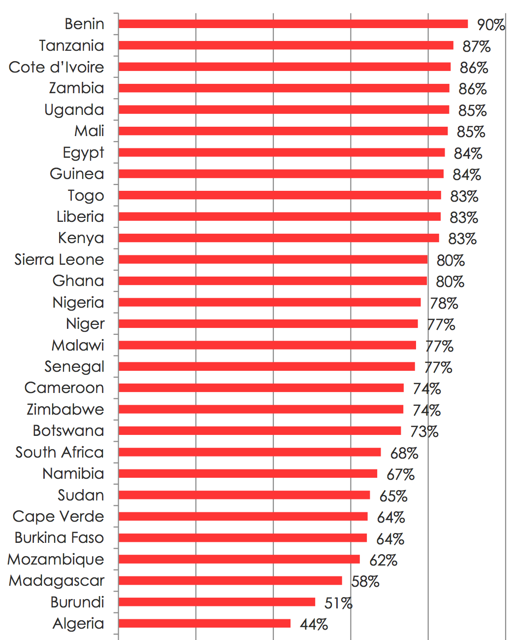
Term limits appear to be popular
Many people in Africa
support term limits
for their president
(surveyed in 2011-2013)
Source: Figure 1 of Dulani (2015)
Term limits appear to be popular (cont.)
Evidence on the impact of term limits
Pioneering study: Besley and Case (1995 QJE)
for US governors during 1950-1986
See Besley and Case (2003 JEL) and Alt et al. (2011 J of Politics) for follow-up
Term limit
Tax revenue
& Govt spending
Evidence on the impact of term limits (cont.)
Some US states move from one-term limit to two-term limit
One-term limit
Two-term limit
No incentive
Incentive
No incentive
Elected once
Elected twice
What's the benefit of term limits?
The baseline political agency model suggests
only a negative impact of term limits on citizens' welfare
Is there any situation where term limits enhance welfare?
Smart and Sturm (2013) extend the political agency model
to tackle this issue
Here we follow Section 3.4.3 of Besley (2006)
Extending the baseline model
In the baseline model, voters know \(e_t=1\) is a good policy
Now assume that voters are unsure about which is a good policy
To formally model this uncertainty, introduce a state of the world:
s_t\in\{0,1\}
And voters' payoff is given by
\Delta
0
if \(e_t = s_t\)
if \(e_t \neq s_t\)
But voters do not know \(s_t\)
Voters prior belief on \(s_t\)
\Pr(s_t=0)=1/2
At the election, voters observe \(e_1\)
But citizens' payoff from \(e_1\) doesn't realize yet
When choosing policy, the incumbent observes \(s_t\)
Extending the baseline model (cont.)
The congruent politician's preference: the same as voters
The dissonant politician's preference:
\Delta
0
if \(e_t = s_t\)
if \(e_t \neq s_t\)
r_t
0
if \(e_t = 1\)
if \(e_t = 0\)
e.g. \(e_t=1\) pleases an interest group, but could also benefit the whole population
Extending the baseline model (cont.)
Timing of Events
Period 1
1
Nature picks:
The incumbent politician observes these while voters do not
the type of the incumbent politician \(i \in \{c,d\} \)
the state of the world \(s_1\in \{0,1\} \)
the rent for dissonant politician \(r_1 \sim G(\cdot)\)
2
The incumbent politician chooses policy \(e_1 \in \{0,1\}\)
Period 1 payoffs realize for incumbent, but not for voters
Timing of Events (cont.)
Election
3
Voters decide whether to re-elect the incumbent
But voters do not observe it
4
Nature picks the type of opposition candidate
Timing of Events (cont.)
5
The winning politician chooses policy \(e_2 \in \{0,1\}\)
Period 2
All payoffs realize and the game ends.
6
Nature picks:
the state of the world \(s_1\in \{0,1\} \)
the rent for dissonant politician \(r_1\)
Analysis
Among possibly many equilibria, focus on the one in which:
Congruent incumbent picks \(e_1 = 0 \) regardless of \(s_1\)
Dissonant incumbent picks \(e_1 = 0 \) if \(r_1 < \beta(E+\mu)\)
Voters re-elect the incumbent if and only if \(e_1=0\)
That is, when the re-election incentive backfires
We now derive the condition under which this is an equilibrium
picks \(e_1 = 1 \) otherwise
Voters optimization
They prefer electing a congruent politician for period 2
Probability of being congruent:
\frac{\pi}{\pi+(1-\pi)G(\beta(E+\mu))}>\pi
Opposition
Incumbent delivering \(e_1=0\)
It's optimal to re-elect the incumbent if \(e_1=0\)
\Delta > \frac{1}{2}\Delta
if dissonant
if congruent
Dissonant incumbent's optimization
For the same reason as in the baseline model, it's optimal to pick
\(e_1 = 0 \) if \(r_1 < \beta(E+\mu)\)
\(e_1 = 1 \) otherwise
Congruent incumbent's optimization
Given that he'll be re-elected by choosing \(e_1=0\),
it's clearly optimal to choose \(e_1=0\) if \(s_1=0\)
If \(s_1=1\), his payoff is
if picking \(e_1=0\) (and re-elected)
\beta(E+\Delta)
\Delta
if picking \(e_1=1\) (and kicked-out)
So it's optimal to choose \(e_1=0\) even if \(s_1=1\) when
E>\frac{(1-\beta)\Delta}{\beta}
An equilibrium
Congruent incumbent picks \(e_1 = 0 \) regardless of \(s_1\)
Dissonant incumbent picks \(e_1 = 0 \) if \(r_1 < \beta(E+\mu)\)
Voters re-elect the incumbent if and only if \(e_1=0\)
The following strategy profile:
is a Perfect Bayesian Equilibrium under the condition
\(e_1 = 1 \) otherwise
E>\frac{(1-\beta)\Delta}{\beta}
If the incumbent is term-limited in period 1
Congruent incumbent picks \(e_1 = s_1 \)
Dissonant incumbent picks \(e_1 = 1 \)
Probability of congruent politician in office: \(\pi\)
In both periods:
Voters' welfare w/ and w/o term limit
\pi \Delta + (1-\pi) \frac{1}{2}\Delta
if term-limited
if not term-limited
Period 1 (Incentive effect)
\frac{1}{2}\Delta
Term limit increases welfare by
\frac{\pi}{2}\Delta
Voters' welfare w/ and w/o term limit
\pi \Delta
if term-limited
if not term-limited
Period 2 (Selection effect)
Term limit decreases welfare by
(1-\pi)(1-\lambda)\frac{\pi}{2}\Delta
+ (1-\pi) \lambda \frac{1}{2} \Delta
\lambda \equiv G(\beta(E+\mu))
+ (1-\pi) (1-\lambda) \pi\Delta
+ (1-\pi) (1-\lambda) (1-\pi)\frac{1}{2} \Delta
\pi \Delta + (1-\pi) \frac{1}{2}\Delta
where
Voters' welfare w/ and w/o term limit
decreases welfare by
\beta(1-\pi)(1-\lambda)\frac{\pi}{2}\Delta
Term limit
increases welfare by
\frac{\pi}{2}\Delta
Net effect
[1-\beta(1-\pi)(1-\lambda)]\frac{\pi}{2}\Delta > 0
Implications
Term limit can increase welfare when
Being in office is too attractive for congruent politicians
i.e. the equilibrium condition:
Citizens do not observe the policy outcome before elections
expect a particular policy to be better (\(e_1=0\))
using a similar version of the political agency model,
discuss when policy-making should be delegated to "judges"
E>\frac{(1-\beta)\Delta}{\beta}
(Related) Evidence
US state governors are more likely to implement
environment-friendly policies in two cases:
when term-limited in brown states
when not term-limited in green states
Other
Applications
Political business cycles
use a version of political agency model (cf. Section 3.4.4 of Besley 2006)
Policy decisions twice within Period 1
But the second policy's outcome is unobserved at the election
to derive the electoral cycle in public investment
Evidence
Shi and Svensson (2006) for cross-country evidence
Akhmedov and Zhuravskaya (2004 QJE) for Russian regions
Cole (2009) for Indian states
The role of media
extend the political agency model in which
They show that disaster relief by Indian states is larger
for states with many people subscribing to newspapers
the probability of learning the policy outcome
increases with the presence of mass media
Optimal tax policy if politicians are corruptible
Allow government to issue debt in the presence of aggregate shocks
Acemoglu, Golosov, Tsyvinski (2008 Econometrica)
In a neoclassical growth model with non-stationary voting strategy and without any restriction on tax instruments
Theoretical applications
Incorporate with citizen-candidate model
Autocracy
Extend the model by replacing citizens with the ruling elite
If replacing the leader also causes the ruling elite to lose power
they cannot discipline the leader
Political agency model can incorporate
non-electoral removals of national leaders
Polarization & the disciplining effect of election
If some groups of voters always vote for the opposition
it's less rewarding for the dissonant incumbent to restrain
Disenfranchising such opposition supporters
may therefore improve the quality of government
See Besley and Kudamatsu (2008) for formal argument
e.g. Pak Chunghee in South Korea in 1963
e.g. ethnic allegience
For evidence from India, see Banerjee and Pande (2009)
Causes of democratization
Why politicians have an incentive to hold elections regularly
When citizens are willing to replace the incumbent with less experienced opposition candidate
Summary
Citizens punish the incumbent
if his/her performance is worse than expectation
Given this behavior of citizens
Incumbent restrains from shirking, being corrupt, etc.
Two implications from political agency model
1
2
Both are empirically supported
in the context of Brazilian mayors' corruption
The model can be extended to analyze various policy issues where citizens and politicians are in conflict
Announcement
on
Political Economics II
By 8 December (the first lecture)
Buy a copy at COOP
Read Chapters 1-5

Take note of your questions
to ask during the first lecture
Scheduling
Term Paper
Workshop
December 1: Last Lecture
December 15: Submission deadline (9 am)
December 8: Political Economics II Lecture 1 on empirical methods
December 11 (Mon) or 12 (Tue): Workshop?
18 (Mon)
December 6: My office hour (16:20-17:50)
December 13: My office hour (16:20-17:50)
Political Economics lecture 4: Political Agency Model
By Masayuki Kudamatsu


