Models of Voter Turnout
Lecture 6 Part B, Political Economics 1
OSIPP, Osaka University
24 November, 2017
Masa Kudamatsu
This lecture follows Section I.1.i of Steve Coate's lecture note
Empirical studies will be covered in Political Economics II
See also the survey of theories by Feddersen (2004)
Paradox of Not Voting
We have so far assumed that voters never abstain
This is clearly too strong an assumption
But explaining why people vote is very difficult
Your vote almost never changes the election result
Then why not earn a wage or enjoy leisure time
instead of going to poll?
Unifying framework
A voter's payoff is given by
V_A
V_B
Consider an election with candidates A and B
if candidate A wins
if candidate B wins
Without loss of generality, assume \(V_A > V_B \) and define
\Delta V \equiv V_A - V_B
Going to the polling station costs
C
Bad weather / Distance to polling station
Voter registration
Time required to think which candidate to vote
Unifying framework (cont.)
D
A voter may also derive the consumption value of voting
A sense of civic duty
Meeting friends at the polling station (e.g. Funk 2010)
Then it's optimal to go to poll if
p_A\Delta V + D - C > 0
Probability that a single vote for \(A\) will change the election outcome so that \(A\) wins
p_A
Unifying framework (cont.)
The pivotal voter model
Assume \( D = 0 \)
and endogenize \(p_A\)
The ethical voter model
Assume \( D > 0 \) for some voters
and allow \(p_A\) to be zero
p_A\Delta V + D - C > 0
The Pivotal Voter Model
Model: Players, payoffs, and information
\(n\) voters, each indexed by \(i \in \{1, ..., n\} \)
Each voter can be either of the two types: A's supporter or B's
The types of other voters are unknown to each voter
A's supporter earns a benefit of \(b\) if A wins
B's
\(x\) if B wins
Probability of being A's supporter is \(\mu\)
The cost of voting for voter \(i\) is given by \(c_i \sim F(c_i)\)
It's not observed by other voters
(\(n\) is an even number)
Model: Election
Each voter decides
whether to vote their preferred candidate or to abstain
A wins if [# of votes for A] \(\geq\) [# of votes for B]
B wins otherwise
Analysis: Equilibrium concept
The model is a static game of incomplete information
Every voter simultaneously decide whether to vote
without knowing other voters' preference type and voting cost
Define a voter's strategy (whether to vote)
as a function of their preference type and voting cost
We solve the model for Bayesian Nash Equilibrium in which
Each voter's strategy is the best response to each other
Focus on a symmetric equilibrium
Each preference type uses the same strategy
Analysis: Cut-off strategy
Voter \(i\) of preference type A votes if
p_A b\geq c_i
B
p_B x\geq c_i
Each type thus uses the cut-off strategy
Type \(\tau \in \{A,B\} \) picks the cutoff value, \(\gamma_\tau\),
so that voter \(i\) goes to vote if and only if \(c_i \leq \gamma_\tau\)
A symmetric equilibrium is then characterised
by a pair of the optimal cut-off values, \(\gamma^*_A, \gamma^*_B \)
Analysis: Each voter's optimal strategy
Suppose all the other \(n-1\) voters follow the equilibrium strategy \(\gamma^*_A, \gamma^*_B \)
Let \(\rho (\nu_A, \nu_B; \gamma^*_A, \gamma^*_B) \) denote the probability that
out of the \(n-1\) voters, \(\nu_A\) vote A and \(\nu_B\) vote B
If voter \(i\) is type A, his/her vote matters with probability
\sum_{\nu=1}^{n/2} \rho (\nu-1, \nu; \gamma^*_A, \gamma^*_B)
In the equilibrium we have
\gamma^*_A = b \sum_{\nu=1}^{n/2} \rho (\nu-1, \nu; \gamma^*_A, \gamma^*_B)
Analysis: Each voter's optimal strategy
Similarly, if voter \(i\) is type B, his/her vote is pivotal with probability
\sum_{\nu=0}^{n/2-1} \rho (\nu, \nu; \gamma^*_A, \gamma^*_B)
In the equilibrium we have
\gamma^*_B = x \sum_{\nu=0}^{n/2-1} \rho (\nu, \nu; \gamma^*_A, \gamma^*_B)
Analysis: Equilibrium
A pair of \(\gamma_A^*, \gamma_B^*\) that satisfy
constitutes a symmetric equilibrium
\gamma^*_B = x \sum_{\nu=0}^{n/2-1} \rho (\nu, \nu; \gamma^*_A, \gamma^*_B)
\gamma^*_A = b \sum_{\nu=1}^{n/2} \rho (\nu-1, \nu; \gamma^*_A, \gamma^*_B)
where \(\rho (\nu_A, \nu_B; \gamma^*_A, \gamma^*_B) \) is given by...
Probability that \(s\) of \(n-1\) voters are type A
P(s)\equiv{{n-1}\choose{s}}\mu^s(1-\mu)^{n-1-s}
Probability that \(\nu_s\) of \(s\) voters of type A go to poll
A(s,\nu_s,\gamma_A^*)\equiv{{s}\choose{\nu_s}}F(\gamma^*_A)^{\nu_s}(1-F(\gamma_A^*))^{s-\nu_s}
Probability that \(\nu_o\) of \(n-1-s\) voters of type B go to poll
B(s,\nu_s,\gamma_B^*)\equiv{{n-1-s}\choose{\nu_o}}F(\gamma^*_B)^{\nu_o}(1-F(\gamma_B^*))^{n-1-s-\nu_o}
Then the probability of being pivotal is given by
\rho (\nu_A, \nu_B; \gamma^*_A, \gamma^*_B)
=\sum_{s=\nu_A}^{n-1-\nu_B}A(s,\nu_A,\gamma^*_A)B(s,\nu_B,\gamma^*_B)P(s)
Implication: Paradox of not voting
As \(n\) gets very large (as in national elections)
\gamma^*_B = x \sum_{\nu=0}^{n/2-1} \rho (\nu, \nu; \gamma^*_A, \gamma^*_B)
\gamma^*_A = b \sum_{\nu=1}^{n/2} \rho (\nu-1, \nu; \gamma^*_A, \gamma^*_B)
\gamma^*_A, \gamma^*_B
converge to zero
(Bayesian)
Nash Equilibrium
\gamma^*_B
\gamma^*_A
\gamma^*_B
\gamma^*_A
As \(n\) goes up
Converge to zero
Limitation
Even in large elections, many people do vote
For this to be consistent with the pivotal voter model,
the cost of voting must be zero
But then it cannot explain variation in turnout across elections
So we have to allow \(D > 0\) in the condition for going to poll:
p_A\Delta V + D - C > 0
Ethical Voting Model
Civic duty
One source of \(D > 0\) from voting is
warm glow from doing one's duty as a citizen
(or avoiding feeling guilty of failing to do it)
A way to model this idea is to assume rule-utilitarian citizens
Rule-utilitarians
Follow the rule that maximizes social welfare if everyone else also follows the same rule
e.g.
Do not throw rubbish in the street
Do not pick a flower from park
The ethical voter model incorporates this idea
into a model of voter turnout
Overview of the model
Two groups of citizens
Each supports one of the two candidates/parties, or
Those in favor of and against a proposal in a referendum
Each wants to increase the probability of winning in majority voting
But also wants to minimize the total cost of voting borne by citizens
Overview of the model (cont.)
Some citizens in each group: rule-utilitarian
Set the rule that minimizes the social cost of voting
if everyone else follows the same rule
The rule in this model:
Go to poll if their cost of voting does not exceed a threshold
The higher the threshold, the higher turnout from the group
Turnout
of your own group
Marginal
benefit/cost
Marginal gain in winning probability
declines with turnout
Overview of the model (cont.)
Turnout
of your own group
Marginal
benefit/cost
Marginal social cost of voting
increases with turnout
because
those citizens with smaller cost of voting go to poll first
Overview of the model (cont.)
Turnout
of your own group
Marginal
benefit/cost
Optimal
turnout
Overview of the model (cont.)
Turnout
of your own group
Marginal
benefit/cost
Turnout
goes up
If the other group turn out more
Overview of the model (cont.)
The other group's
turnout
Your group's turnout
(Bayesian)
Nash Equilibrium
Overview of the model (cont.)
Formal model
Here we follow Feddersen and Sandroni (2006)
Differences from Coate and Colin (2004) will be mentioned
Players
A continuum of citizens with two preference types
Fraction \(k\) prefers candidate 1; \(1-k\) candidate 2
k\in(0,\frac{1}{2}]
measure the degree of polarization
Fraction \(\tilde{q}_i\) for group \(i\in\{1,2\}\): ethnical voters
\tilde{q}_i
uniformly distributed in [0,1]
This uncertainty assures the existence of the equilibrium
Coate and Collin (2004) assume instead every citizen is ethical, which implies no equilibrium may exist
Preference for social outcomes
Type 1 citizens:
pw-\phi
Type 2 citizens:
(1-p)w-\phi
p
Winning probability for candidate 1
w
Importance of the election
\phi
Expected social cost of voting
Coate and Colin (2004) instead assume
the total cost of voting for their own group matters
Coate and Colin (2004) allow this to differ across types
Preference over voting
-x \bar{c}
x
\bar{c}
Maximum individual cost of voting
if voting
0
if abstaining
Individual cost of voting as a share of the maximum
For both ethical and non-ethical voters:
Uniformly distributed over \((0,1)\)
If the model completes here
we have zero turnout in the equilibrium
Each citizen's single vote does not affect \(p\)
Voting is costly
Ethical voters
Fraction \(\tilde{q}_i\) for group \(i\in\{1,2\}\): ethnical voters
\tilde{q}_i
uniformly distributed in [0,1]
This uncertainty assures the existence of the equilibrium
Coate and Collin (2004) assume instead every citizen is ethical, which implies no equilibrium may exist
Ethical voters' preference over voting
They derive a payoff of
D (> \bar{c})
If behaving according to the group's "rule"
Otherwise
0
The group's rule
Vote if and only if
x \leq \sigma_i
(i\in\{1,2\})
Ethnical voters' action
Set the cutoff value of the individual cost of voting:
\sigma_i \in [0,1]
Non-ethnical voters' action
Decide whether to go to poll
Everyone abstains
Analysis: Expected social cost of voting
kE(\tilde{q}_1)\int_0^{\sigma_1} x\bar{c} d x
For group 1:
Expected #
of ethnical voters
in group1
E(\tilde{q}_1)=\frac{1}{2}
Expected fraction of ethical voters among group 1:
\(\tilde{q}_1\) distributed uniformly over [0,1]
Analysis: Expected social cost of voting
For group 1:
Expected #
of ethnical voters
in group1
E(\tilde{q}_1)=\frac{1}{2}
Expected fraction of ethical voters among group 1:
\(\tilde{q}_1\) distributed uniformly over [0,1]
(k/2)\int_0^{\sigma_1} x\bar{c} d x
Analysis: Expected social cost of voting
For group 1:
Sum of voting cost
among ethical voters
(k/2)\int_0^{\sigma_1} x\bar{c} d x
Percentile of voting cost
0
1
voting cost
\bar{c}
\sigma_1\bar{c}
\sigma_1
Analysis: Expected social cost of voting
For group 1:
Sum of voting cost
among ethical voters
(k/2)\frac{1}{2}(\sigma_1)^2 \bar{c}
Percentile of voting cost
0
1
voting cost
\bar{c}
\sigma_1\bar{c}
\sigma_1
Analysis: Expected social cost of voting
For group 1:
\frac{k(\sigma_1)^2 \bar{c}}{4}
For group 2:
(1-k)E(\tilde{q}_2)\int_0^{\sigma_2} x\bar{c} d x
=\frac{(1-k)(\sigma_2)^2\bar{c}}{4}
\phi=\frac{\bar{c}}{4}(k(\sigma_1)^2+(1-k)(\sigma_2)^2)
\equiv \phi(\sigma_1, \sigma_2)
Overview of the model (cont.)
Turnout
of your own group
Marginal
benefit/cost
Marginal social cost of voting
increases with turnout
Those citizens with smaller cost of voting go to poll first
Analysis: Winning probability for candidate 1
# of votes for candidate 1
k\tilde{q}_1\sigma_1
# of votes for candidate 1
(1-k)\tilde{q}_2\sigma_2
Candidate 1 wins with probability
\Pr[(k\tilde{q}_1\sigma_1)\geq(1-k)\tilde{q}_2\sigma_2]
=\Pr[\frac{\tilde{q}_2}{\tilde{q}_1}\leq \frac{k\sigma_1}{(1-k)\sigma_2}]
=F(\frac{k\sigma_1}{(1-k)\sigma_2})
where \(F(\cdot)\) is the c.d.f of \(\tilde{q}_2/\tilde{q}_1\)
\equiv p(\sigma_1,\sigma_2)
Overview of the model (cont.)
Turnout
of your own group
Marginal
benefit/cost
Marginal gain in winning probability
declines with turnout
Analysis: Each group's optimal rule
\max_{\sigma_1}p(\sigma_1,\sigma_2)w-\phi(\sigma_1, \sigma_2)
FOC
\frac{k}{1-k}\frac{1}{\sigma_2}f(\frac{k}{1-k}\frac{\sigma_1}{\sigma_2})w\geq \frac{\bar{c}}{2}k\sigma_1
with strict inequality if \(\sigma_1=1\)
Similarly, the FOC for group 2
\frac{k}{1-k}\frac{\sigma_1}{(\sigma_2)^2}f(\frac{k}{1-k}\frac{\sigma_1}{\sigma_2})w\geq \frac{\bar{c}}{2}(1-k)\sigma_2
with strict inequality if \(\sigma_2=1\)
Group 1 solves
Overview of the model (cont.)
The other group's
turnout
Your group's turnout
(Bayesian)
Nash Equilibrium
Closed-form solution
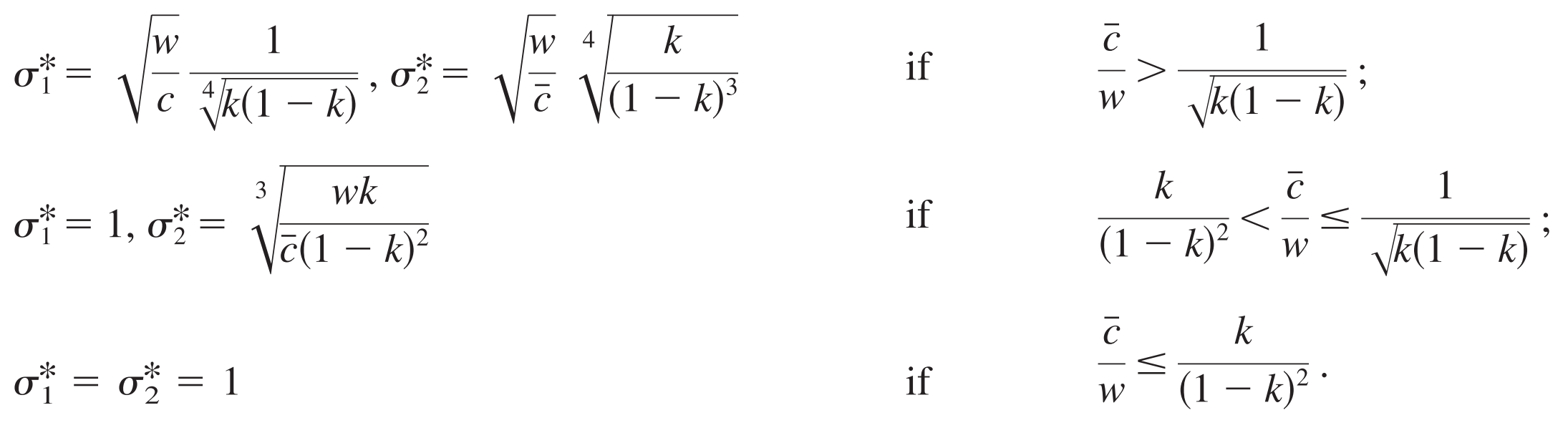
Table 1 of Feddersen and Sandroni (2006)
Comparative statics #1
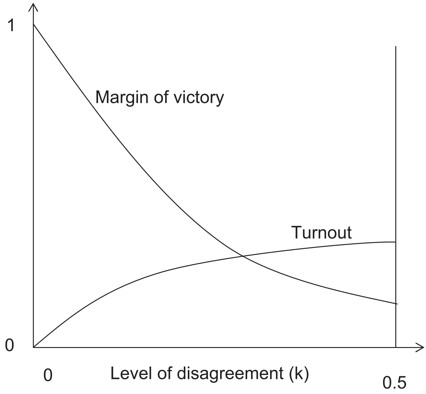
Figure 2 of Feddersen and Sandroni (2006)
Turnout is negatively correlated with margin of victory
Consistent with available evidence
Comparative statics #2
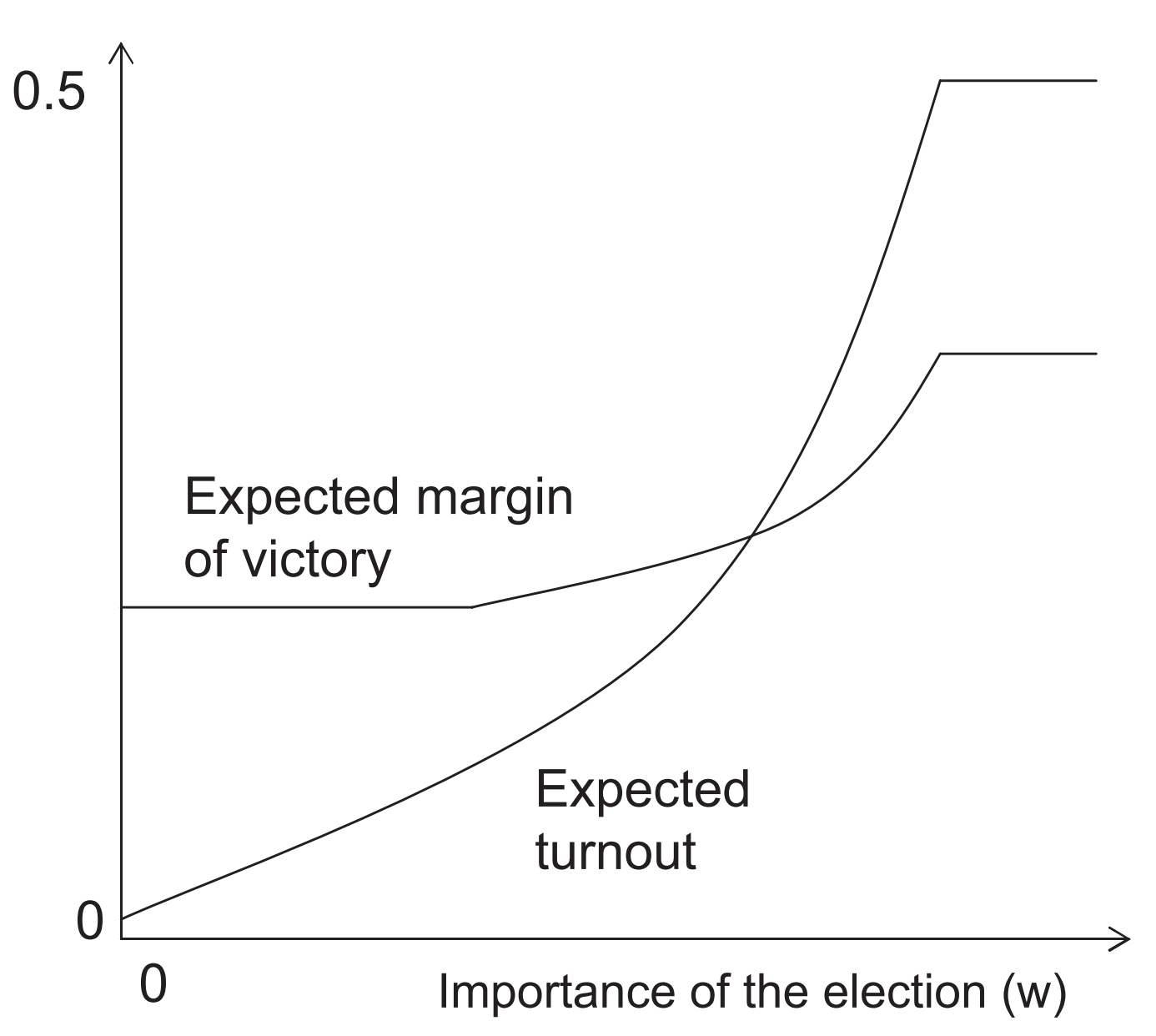
Figure 3 of Feddersen and Sandroni (2006)
Turnout is higher the more important the election
Consistent with available evidence (higher turnout for presidential elections than for state elections in U.S.)
Ethical Voting Model: An Application
Impact of providing candidate information
on urban poor's turnout in India
Policies favoring the poor are rarely adopted in developing countries
Is this because the poor is uninformed about candidates at the election?
e.g. High absenteeism of teachers and doctors (Chaudhury et al. 2006; Bold et al. 2017)
Motivations
Run an RCT in slums of Delhi
Treatment
Provide information on candidates for 2008 state legislative elections
Outcomes
Turnout increased from 57.5% to 59.5%
Votes dropped for worse-performing incumbents
Experiment
To make sense out of these RCT results, the ethical voting model is extended to incorporate information on candidate quality
Model
of which fraction \(\xi\) prefer \(I\), and \(1-\xi\) prefer \(C\)
Fraction \(\mu\) of voters: partisan
Fraction \(1-\mu\) of voters: ethical
Candidates \(I\) (incumbent) and \(C\) ( challenger)
Once in office, produce a payoff of \(y_t\) to ethnical voters
This payoff depends on their competence, \(\theta_X\), for \(X \in \{I, C\}\)
y_t = \theta_X
Observe \(y_1\), \(\theta_I\), \(\theta_C\) with noise
Decide the cutoff \(c^*\) of voting cost \(c \sim U(0,\bar{c})\)
Candidate information provision reduces this noise
Timing of Events
1
2
3
Incumbent \(I\) produces a payoff \(y_1= \theta_I\)
Nature picks
Nature picks noise in information received by ethical voters
Challenger's competence \(\theta_C \sim N(\bar{\theta}_I, \sigma^2_I)\)
For incumbent's competence, \(\eta_I \sim N(0,\sigma^2_{\eta_I}) \)
For challenger's competence, \(\eta_C \sim N(0,\sigma^2_{\eta_C}) \)
For period 1 payoff, \(\varepsilon \sim N(0,\sigma^2_{\varepsilon}) \)
Incumbent's competence \(\theta_I \sim N(\bar{\theta}_I, \sigma^2_I)\)
Information provision reduces \(\sigma^2_{\eta_I}, \sigma^2_{\eta_C}, \sigma^2_\varepsilon \)
Timing of Events (cont.)
4
Ethical voters observe the (noisy) information on
\tilde{y} = y_1 +\varepsilon
\tilde{\theta_I} = \theta_I +\eta_I
\tilde{\theta_C} = \theta_C +\eta_C
Incumbent's performance
Incumbent's competence
Opposition's competence
5
Ethical voters update their belief on \(\theta_I\) and \(\theta_C\)
6
Ethical voters pick the cutoff for voting cost \(c^*\)
Timing of Events (cont.)
7
Nature picks the fraction of partisan voters supporting \(I\)
\xi \sim U(\frac{1}{2}-\bar{\xi}, \frac{1}{2}+\bar{\xi})
8
The winner produces a payoff of \(y_2\)
where \(\bar{\xi} \in (0, \frac{1}{2}) \)
The winner of the election is \(I\) if and only if
\mu\xi + 1[D>0](1-\mu)\frac{c^*}{\bar{c}} \geq \frac{1}{2}
where \(D \equiv E(\theta_I|\tilde{y}, \tilde{\theta_I}) - E(\theta_C|\tilde{\theta_C})\)
9
Optimal turnout
Ethical voters' optimal cutoff value of voting cost is given by
c^*=\min\{\frac{(1-\mu)|D|}{4\mu\bar{\xi}}, \bar{c}\}
The less partisan voters (lower \(\mu\))
The more likely partisan voters are equally split between the two candidates (higher \(\bar{\xi}\))
Turnout is higher (higher \(c^*\)),
Optimal turnout
Ethical voters' optimal cutoff value of voting cost is given by
c^*=\min\{\frac{(1-\mu)|D|}{4\mu\bar{\xi}}, \bar{c}\}
The larger difference in expected competence between the two candidates (higher \(|D|)\)
Turnout is higher (higher \(c^*\)),
And information provision increases \(|D|\)
Digression: Belief updating w/ normally distributed variables
If the true value \(x\) is distributed normally with mean \(\bar{x}\) & variance \(\sigma^2_x\)
Observing its noisy signal
\tilde{x} = x +\varepsilon
where \(\varepsilon \sim N(0,\sigma^2_\varepsilon) \)
updates the belief on \(x\) is given by
x \sim N (h_\varepsilon \tilde{x}+(1-h_\varepsilon)x, h_\varepsilon\sigma^2_\varepsilon+(1-h_\varepsilon)\sigma^2_x)
where
h_\varepsilon = \frac{(1/\sigma^2_\varepsilon)}{(1/\sigma^2_x)+(1/\sigma^2_\varepsilon)}
is the relative precision of signal
Summary
Political Economics lecture 6 part B: Models of Voter Turnout
By Masayuki Kudamatsu


