Literature Review of Gap-filling methods
Weicheng Zhu
Department of statistics
Iowa State university
Outline
- Introduction to satellite data
- Local linear histogram matching
- Kriging/Cokriging
- Neighborhood Similar Pixel Interpolator (NSPI)
- Geostatistical Neighborhood Similar Pixel Interpolator (GNSPI)
- Weighted linear regression (WLR)
- Information cloning
- Spatio-temporal MRF (STMRF)
- The profile-based interpolator (PBI)
- Tempo-Spectral Angle Model (TSAM)
Satellite data
The Landsat Program is a global land-imaging mission managed through a joint effort of the United States Geological Survey (USGS) and the National Aeronautics and Space Administration (NASA), with the objective of providing globally continuous, high-resolution, multispectral data for scientific and educational use.
Landsat program


Landsat program
Landsat sensors
- Landsat 1 - 4: Multi Spectral Scanner (MSS).
- Landsat 5: MSS and Thematic Mapper (TM).
- Landsat 7: Enhanced Thematic Mapper Plus (ETM+). Operating with scan line corrector (SLC) disabled since May 31, 2003.
- Landsat 8: the Operational Land Imager (OLI) and the Thermal InfraRed Sensor (TIRS).
It takes about 16 days to scan the entire earth
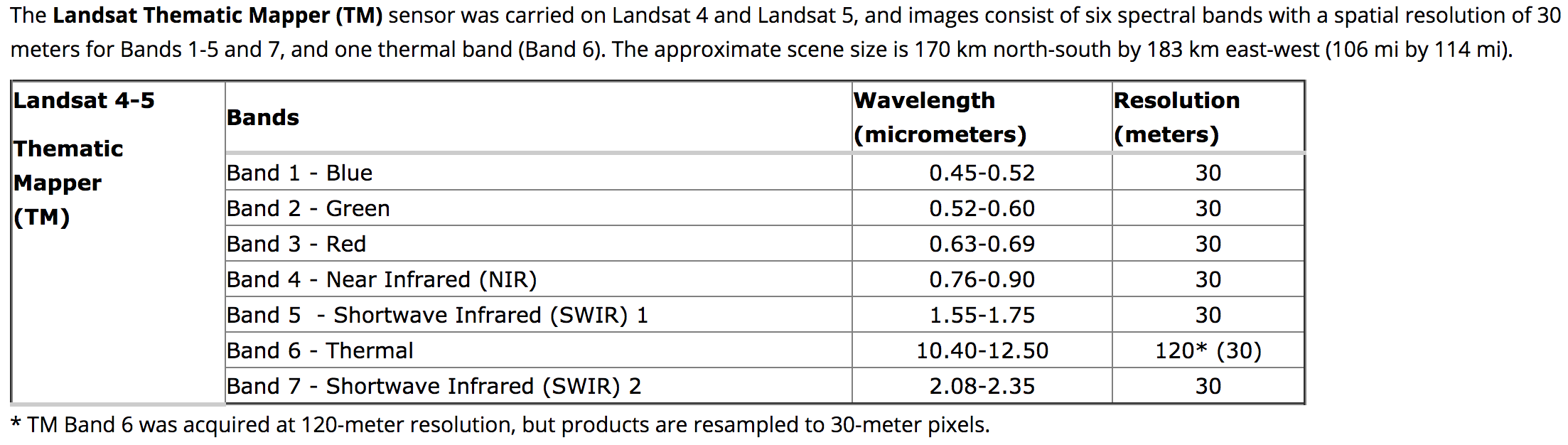
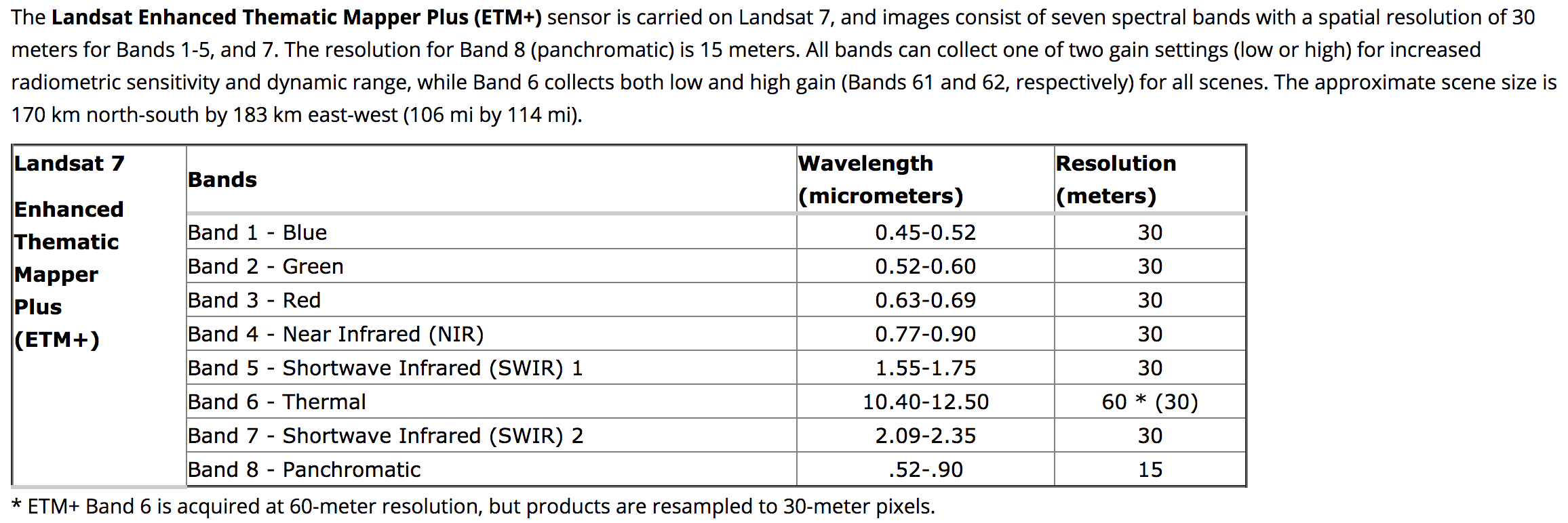
Landsat Bands
MODIS
- Moderate-resolution Imaging Spectroradiometer (MODIS) was launched into Earth orbit by NASA in 1999 on board the Terra (EOS AM) Satellite, and in 2002 on board the Aqua (EOS PM) satellite.
- The instruments capture data in 36 spectral bands at varying spatial resolutions (2 bands at 250 m, 5 bands at 500 m and 29 bands at 1 km).
- Together the instruments image the entire Earth every 1 to 2 days.
- With its low spatial resolution but high temporal resolution, MODIS data is useful to track changes in the landscape over time.
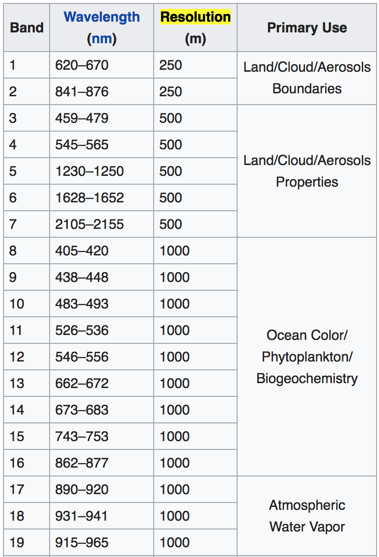
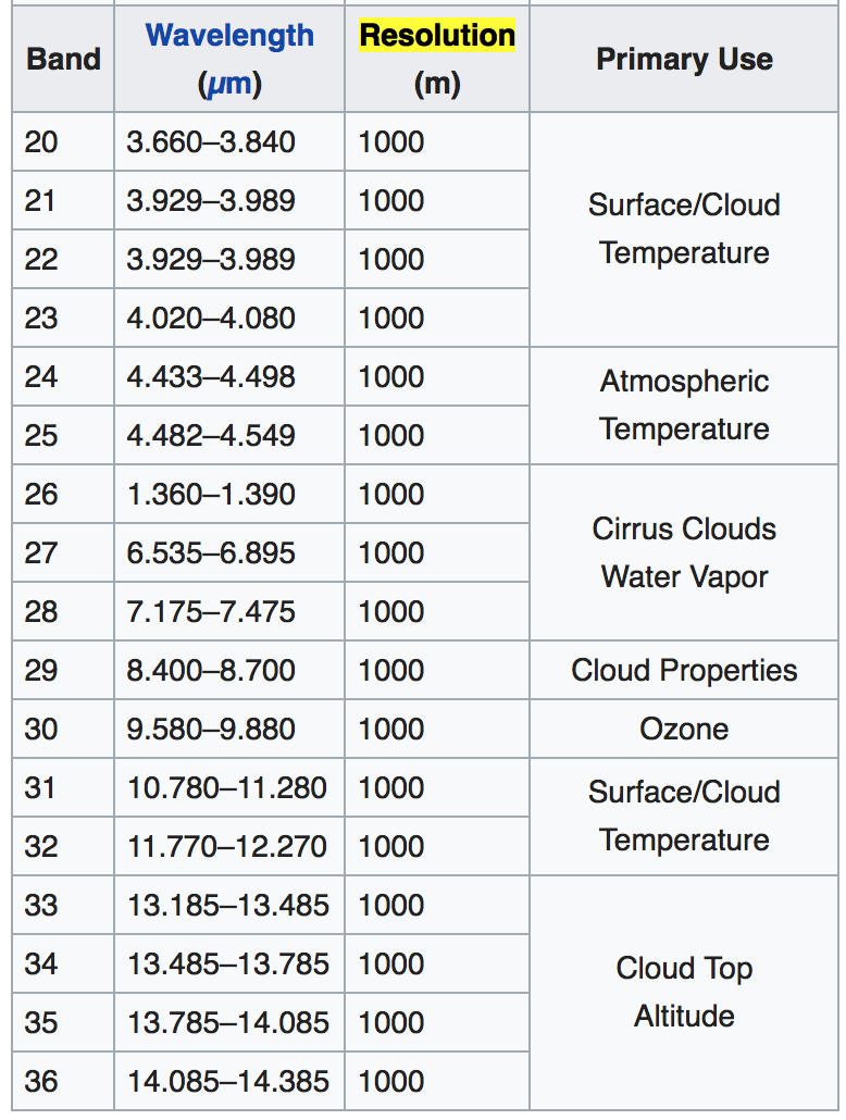
MODIS bands
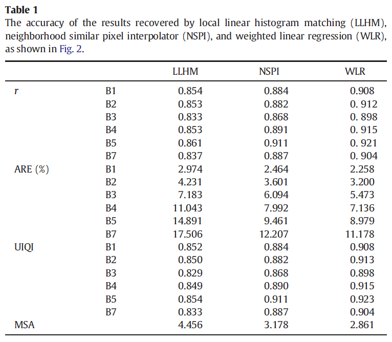
Local linear histogram matching
(LLHM)
SLC-off gap-filled products were released in two phases.
- Phase 1 involved a local linear histogram matching technique that was chosen for rapid implementation. It allowed the user to choose one SLC-on scene for the fill image and was used for gap-filled products generated between 6/1/2004 to 11/18/2004.
- Phase 2 is an enhancement of the Phase 1 algorithm that allows users to choose multiple scenes and to combine SLC-off scenes. Phase 2 processing is used on all gap-filled products processed on or after 11/18/2004.
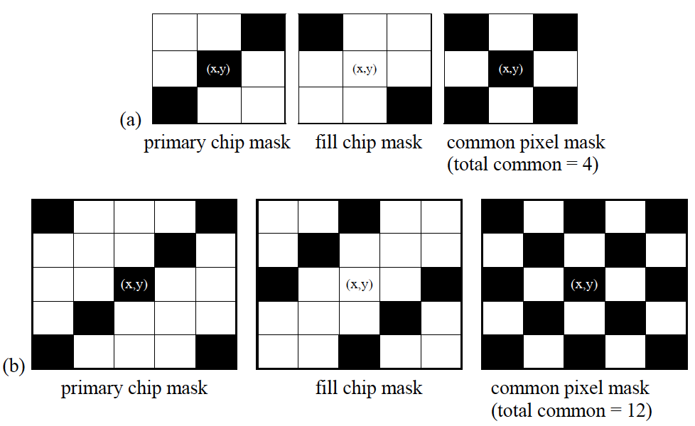
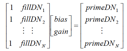
The methodology for creating a histogram-matched composite is to iterate the following process over all gap pixels in the primary scene:
-
Extract an n x n window about the gap pixel in both primary and fill.
-
Find smallest square of pixels
between the two chips that
contains at least a minimum
number of common pixels. - Using the common pixel mask
to extract only the common
pixels from the chip, regress the
primary chip against the fill chip
to find the transform between the
two scenes.
Algorithm
Pros
- Easy to implement
-
satisfactory results in homogenous regions such as forests
Cons
- Need high quality input scenes (e.g., negligible cloud and snow cover)
-
Tend to have difficulty with heterogeneous landscapes
Summary
Kriging/Cokriging
Algorithm

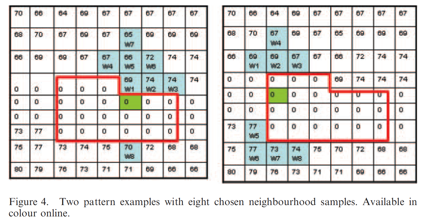
Constrains in choosing neighborhood samplings:
- ensure the close samples (measured by the Euclidean distance)
- make the samples from different sides of the point being estimated if samples have the same closeness.
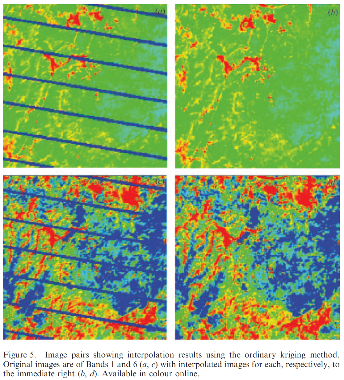
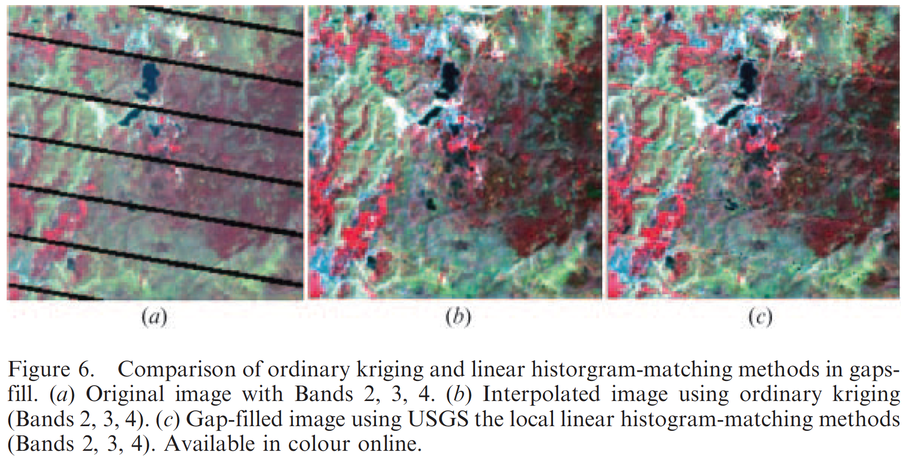
Results
Summary
- Ordinary kriging techniques may provide a powerful tool for interpolating the missing pixels in the SLC-off ETM+ imagery.
- Ordinary cokriging provides little improvement in interpolating the data gap in the SLC-off imagery.
- Need stationarity assumption.
- Relatively slow computation speed.
Complementary Kriging/Cokriging
Due to variability in the locations of un-scanned striations between dates, in many subregions of a target image - particularly near the edges, where striations are relatively wide - secondary information may be more numerous than target data. It is in these sub-regions that cokriging will improve on the predictions of kriging, and will do so with a smaller estimation variance (Goovaerts, 1997; Webster and Oliver, 2001). We therefore contend that kriging and cokriging can be used complementarily to interpolate reflectance at unscanned locations in ETM+ images: cokriging can be implemented by default, but kriging is used in sub-regions of under-sampling. It
is this idea that we follow for geostatistical interpolation.
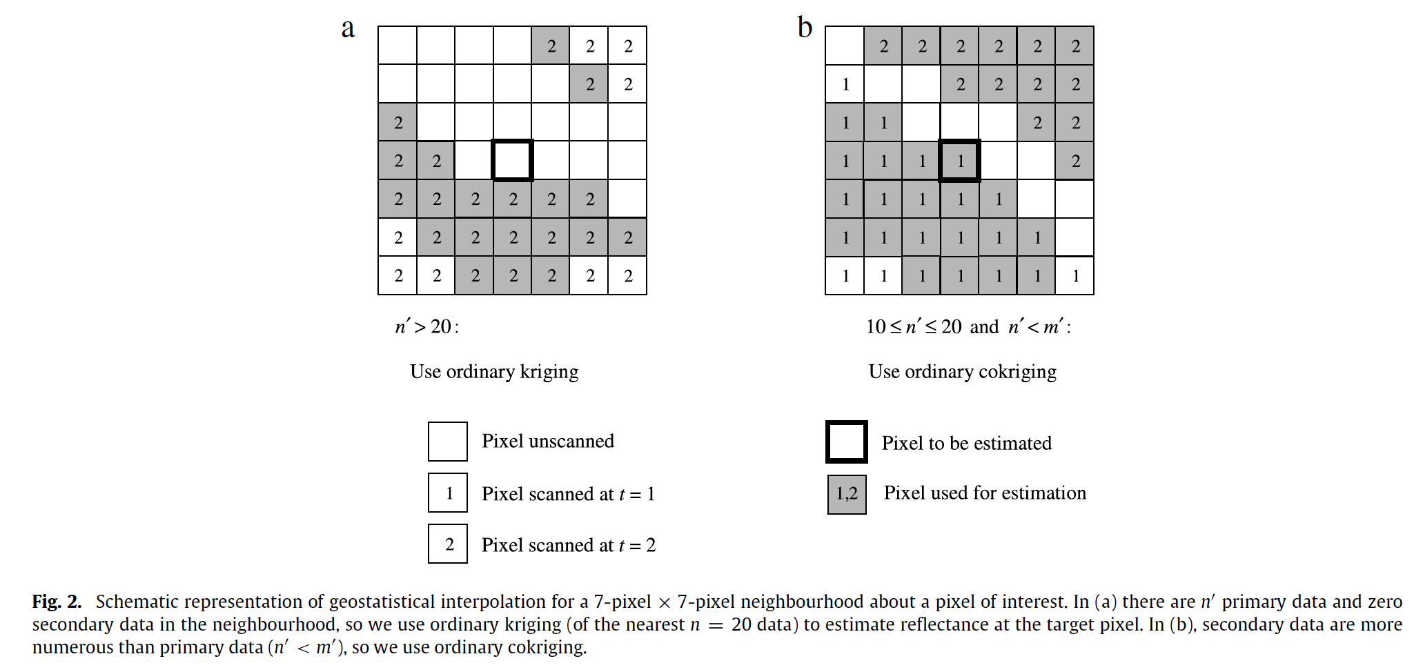
The underlying method is almost the same as Zhang et al., 2007 except that they proposed that kriging and cokriging can be used complementarily to interpolate reflectance at unscanned locations in ETM+ images
Results
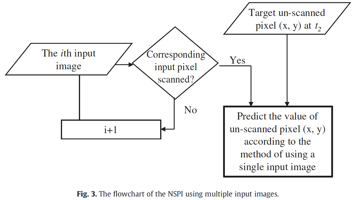
Neighborhood Similar Pixel Interpolator
(NSPI)
There are two data sources that can be used to fill the gaps in target image:
- An appropriate TM image or SLC-on ETM+ image
- SLC-off images acquired at different dates, whereby the scanned parts of these images partly overlap with the gaps in the target image.
Algorithm Using a single TM or SLC-on ETM+ image
1. Selection of neighboring similar pixels.
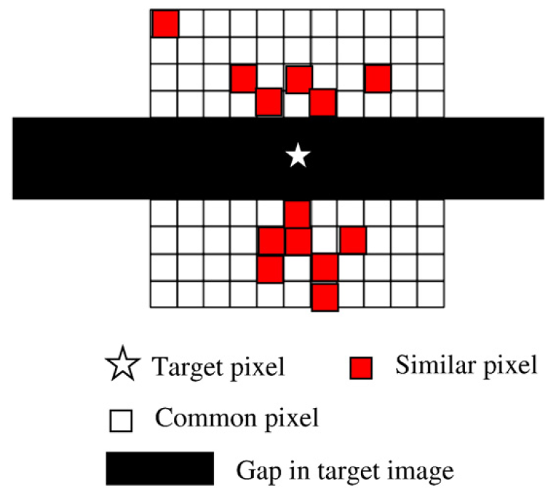
2. Calculation of the weights for similar pixels based on spectral similarity and geographic distance.
3. Calculation of the target pixel value
1. The weighted average of all the similar pixels in the target image.
2. The weighted average of the change provided by
all of the similar pixels is used to calculate the value of the target pixel.

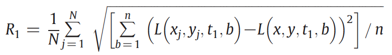


The final predicted value of the target pixel located in the gap is
calculated as:
4. Data quality flag generation

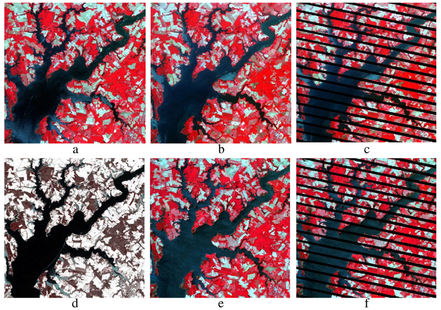
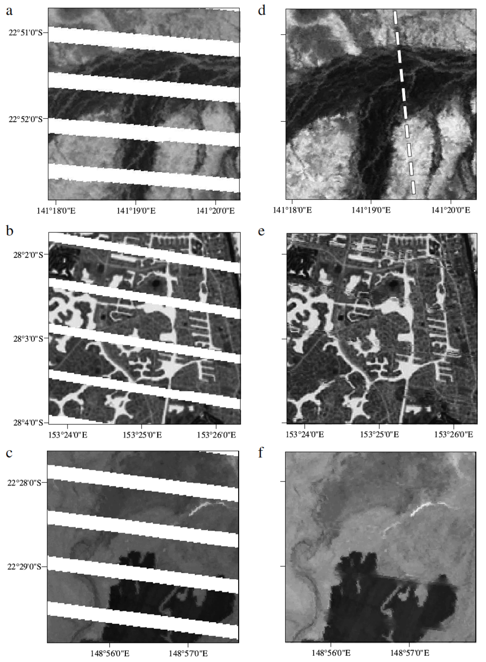
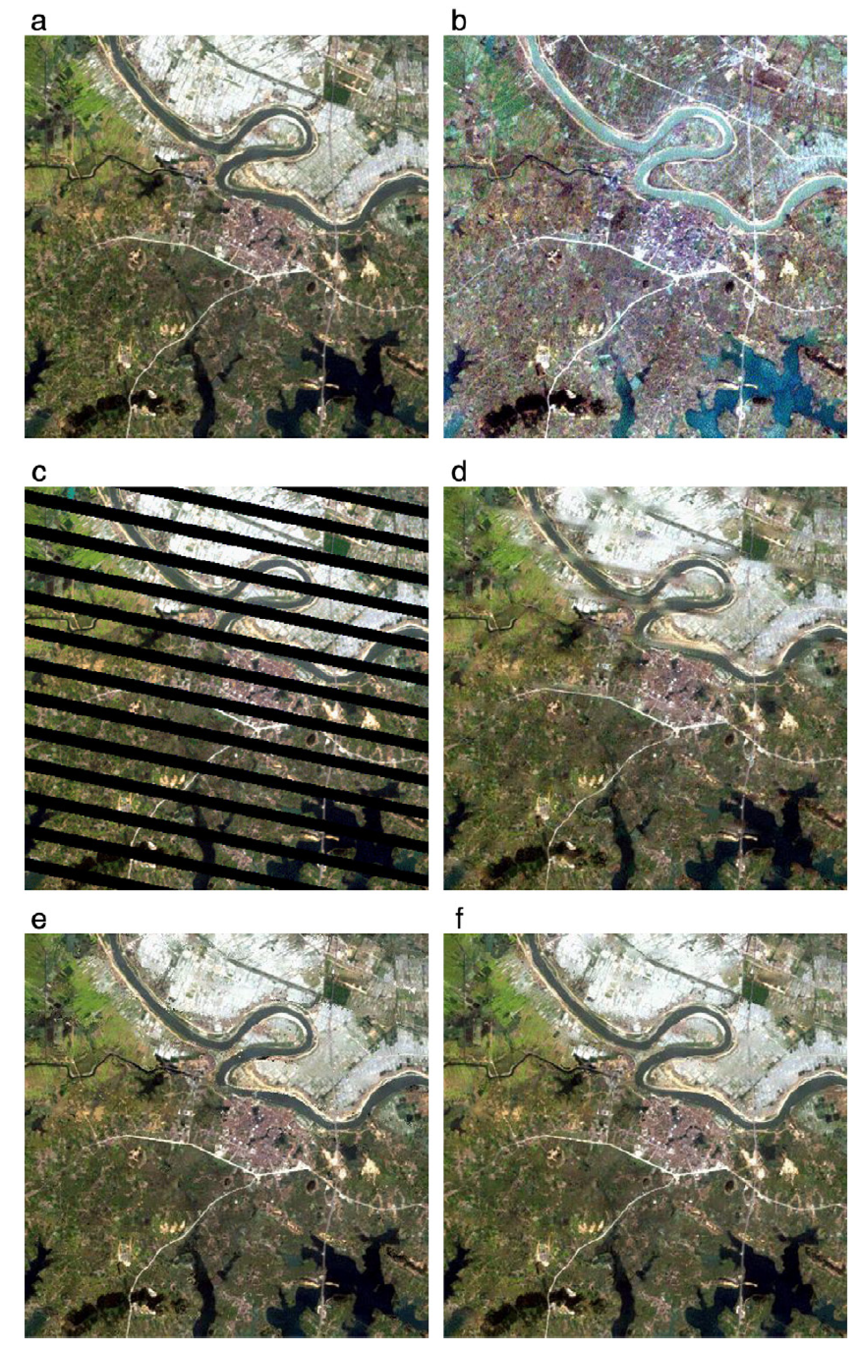
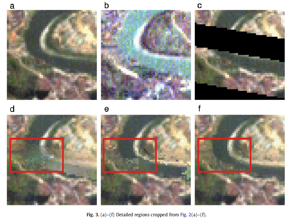
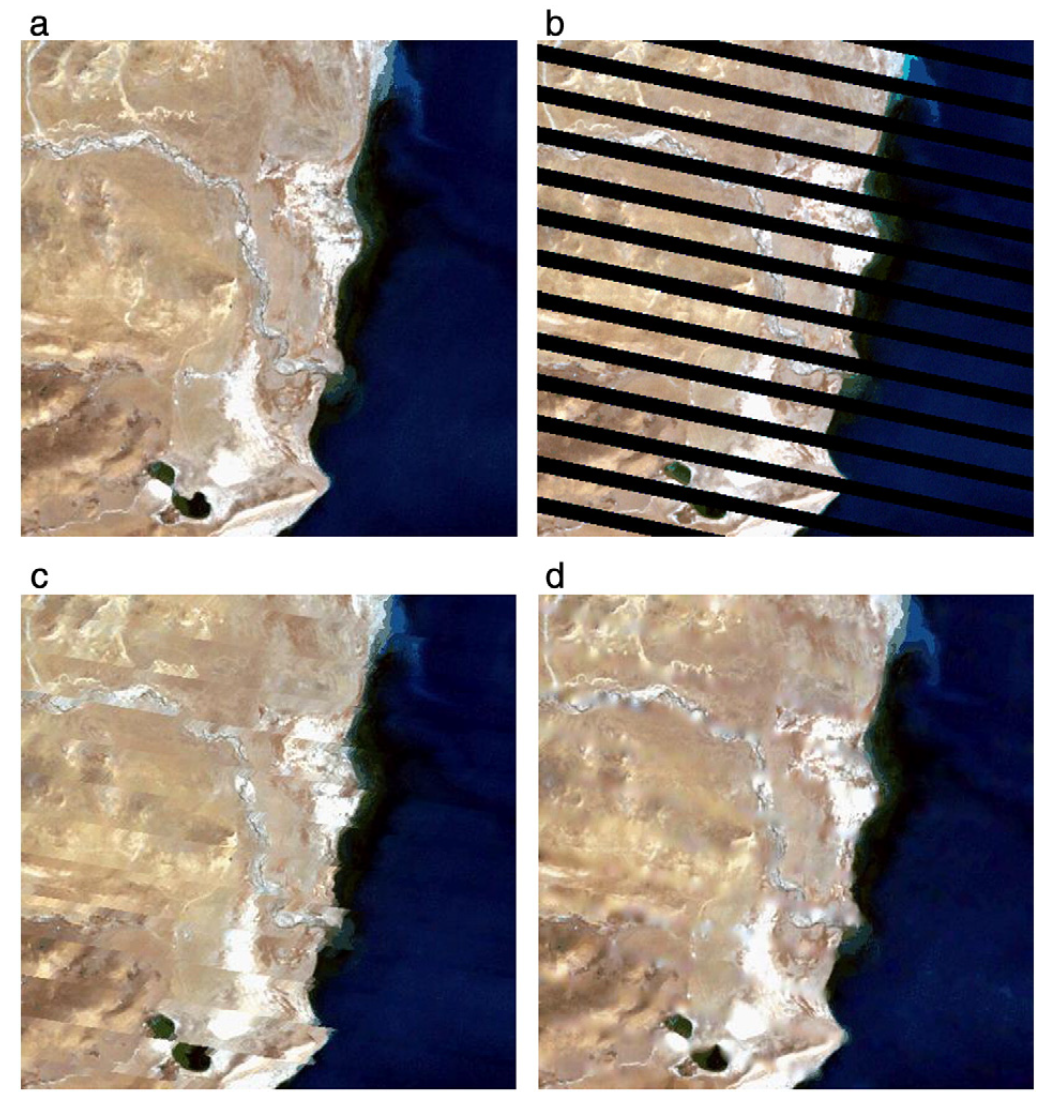
NIR –red –green composites of Landsat TM images for the simulation test for using a single input image. (a) Acquired on May 25, 2008; (b) acquired June 10, 2008; (d) acquired February 8, 2010; (e) acquired April 29, 2010; (c) and (f) SLC-off image were simulated based on (b) and (e) respectively.
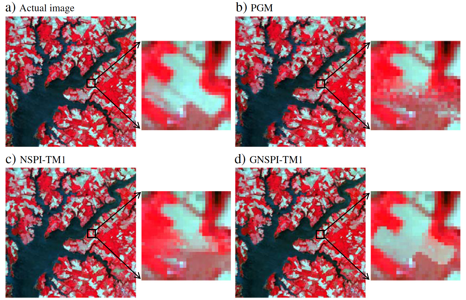
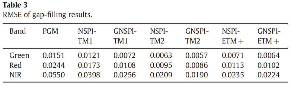
Results
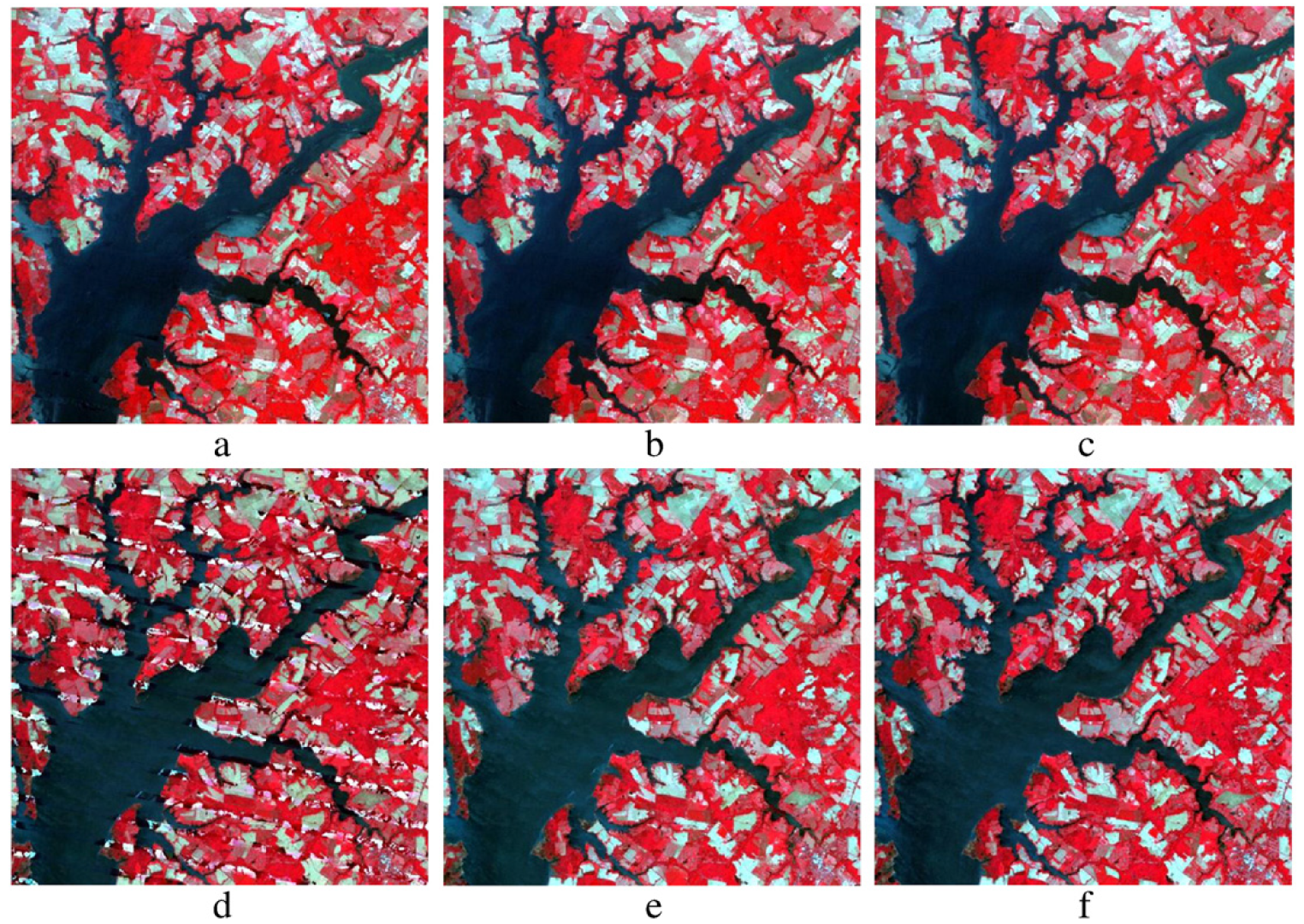
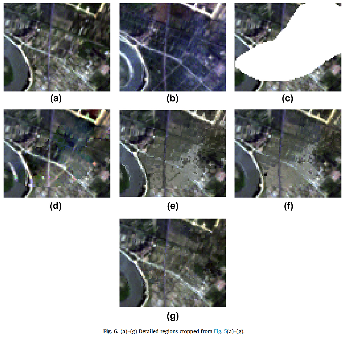
Results of gap-fill for the simulation test of using a single input image. Panels (a) and (b) are the filled images of Fig. 5c by local linear histogram matching and NSPI respectively, and (c) is the actual image; panels (d) and (e) are the filled images of Fig. 5f by local linear histogram matching and NSPI respectively, and (f) is the actual image.
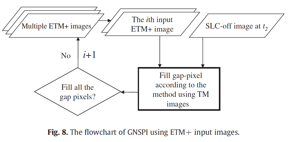
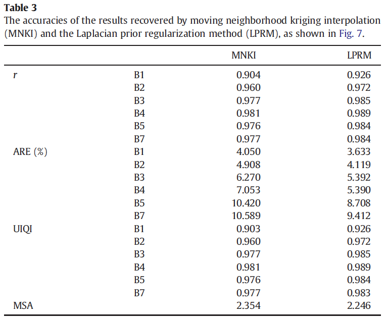
Geostatistical Neighborhood Similar Pixel Interpolator
(GNSPI)
- NSPI is lack of uncertainty of predictions and the impact of changes between input and target images on the final results is not clear.
-
The weight parameters in NSPI are empirically determined by spatial and spectral distances, which may affect their robustness in application for various situations.
-
Geostatistical methods (Pringle et al., 2009; Zhang et al., 2007)
cannot fill the SLC-off images well at the pixel-level, which limits the quantitative applications of these filled images.
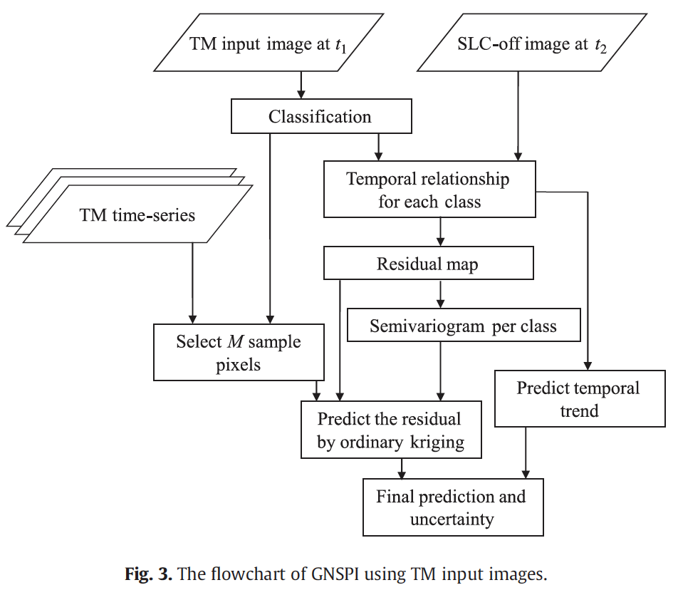
Algorithm Using TM images as input
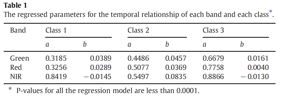
1. Classifying the input image at \(t_1\).
The unsupervised classifier, ISODATA can automatically merge and split classes according to the spectral similarity between pixels to get the optimal classification results (Ball & Hall, 1965).
The date of input image is denoted as \(t_1\) and the date of the target SLC-off image is denoted as \(t_2\).
2. Modeling temporal relationship for each class.
A linear function is used to model the temporal relationship for each class.


3. Modeling semivariogram for each class.
Estimate empirical semivariogram using 1000 random selected pixels for each class.
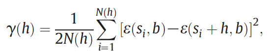
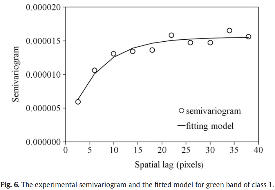
Then fit a parametric semivariogram model:
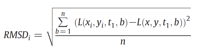
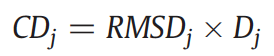
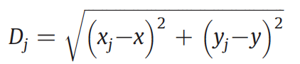
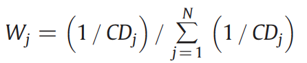
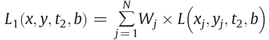
4. Selection of sample pixels. (RMSD as similarity measure)
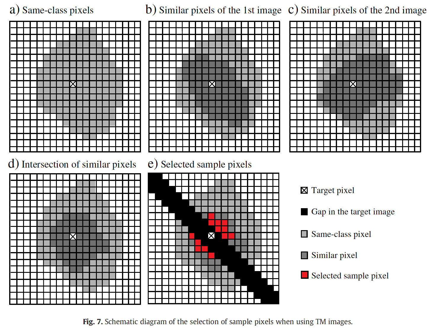
- Based on TM time-series.
- The selected images are temporally separated in one year
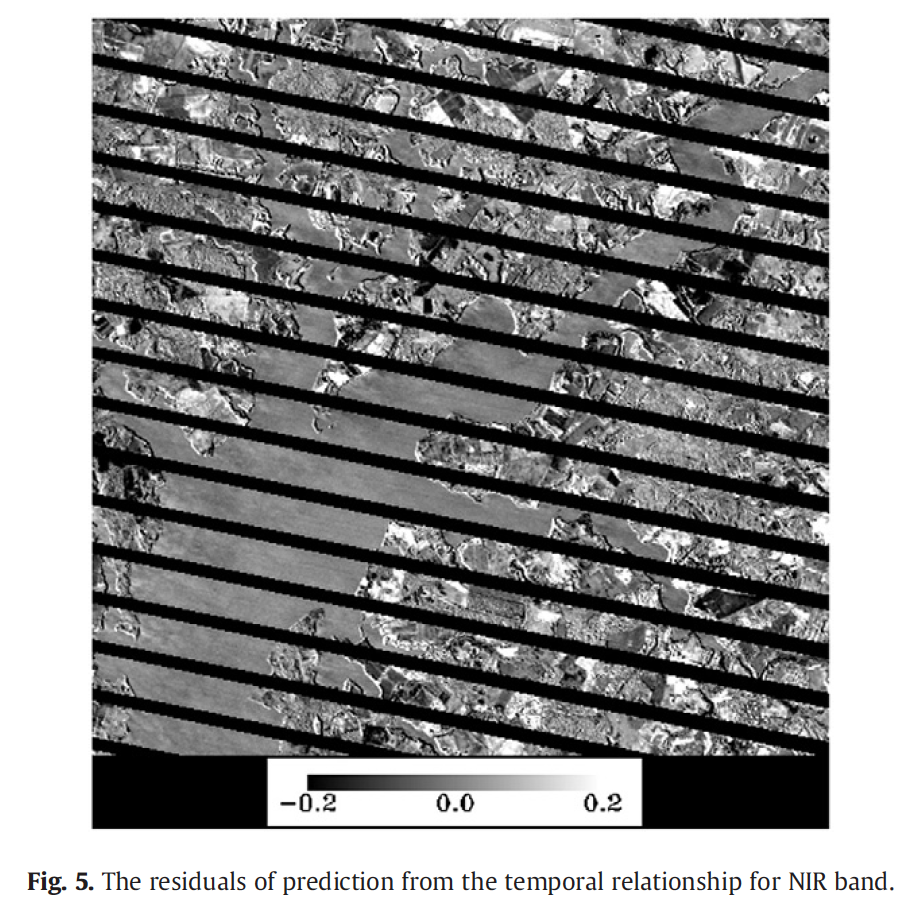
5. Predict the residual of the target pixel by ordinary kriging.
Under the assumption of intrinsic stationarity for the residual image, ordinary kriging predictor is used to estimate the residual value of the target pixel.

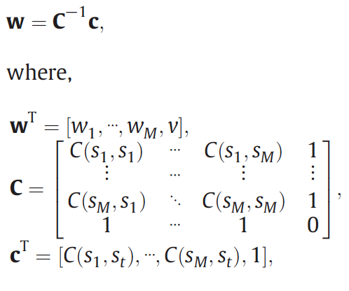
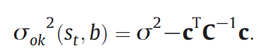
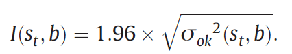
Variance of the ordinary kriging:
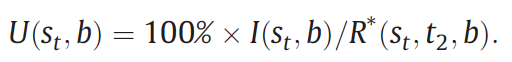
6. Calculate the final prediction and uncertainty.
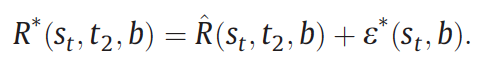
Uncertainty of the final prediction:
Results
Weighted Linear Regression
(WLR)
Two types of recovery methods:
- WLR is used when the inputs are multi-temporal images.
- Non-reference regularization recovery method is used when there are no auxiliary images.
The WLR based on multi-temporal recovery method
1. Select similar pixels of the target location in the primary and fill images, using adaptive threshold values for each target pixel in each band.
2. Calculate weights for selected similar pixels.
3. Fit WLR and do estimation at target pixel.
The regularization based non-reference recovery method
Used when the available images are not sufficient to fill all missing values.
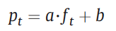
The recovery framework can be written as :
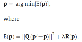
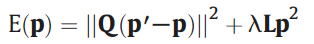
They choose \(R(p)\) to be \(Lp^2\), where \(L\) is the laplacian operator (a second order differential operator in the n-dimensional Euclidean space)
- \(p\)' and \(p\) represent the input primary image and the desired primary image.
- \(Q\) is a diagonal matrix whose diagonal elements are 1 for observed pixels and 0 for unobserved pixels.
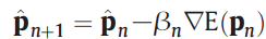
Use he conjugate gradient method to estimate p:
Results for multi-temporal inputs
Results for non-reference method
1. This method cannot restore complicated textures when the invalid area is too large.
2. Relatively slow computing speed.
Cons
Information Cloning
Key idea
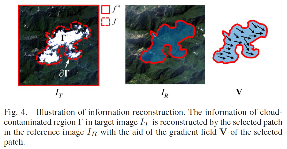
Let \(f\) be unknown image intensity function defined over the cloud-contaminated region, then the problem is converted into a constrained optimization problem.
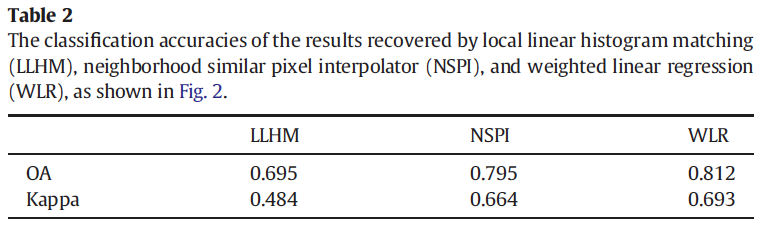
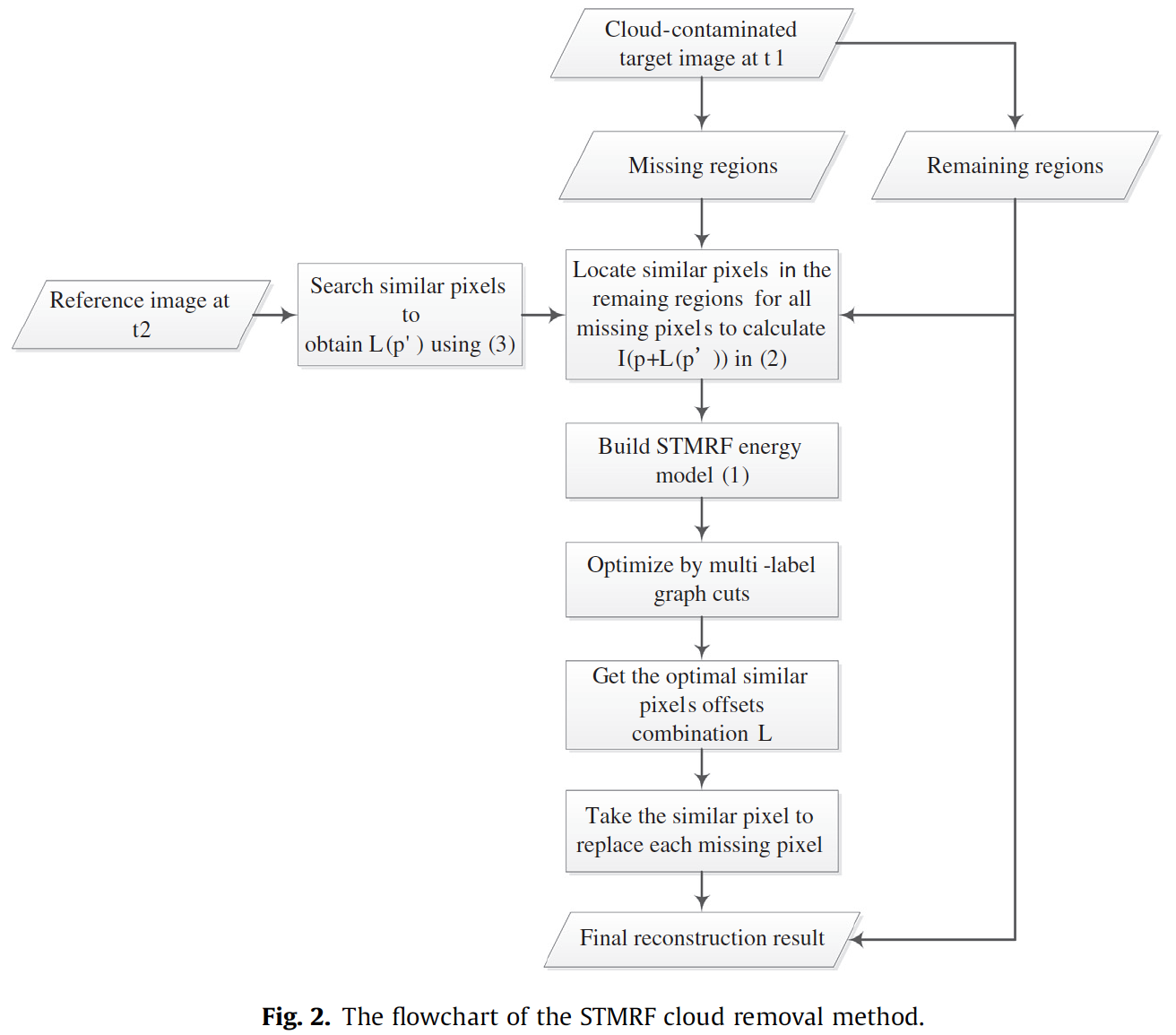
Spatio-temporal MRF
(STMRF)
Cloud removal is essentially an information reconstruction process, and the reconstruction approaches can be grouped into three categories
- noncomplementation approaches; (Applicable for filling small data gaps and not appropriate for large-scale cloud removal.)
- multispectral-complementation based approaches; (Applicable for the removal of haze and thin clouds, and not work for thick cloud removal because thick clouds usually contaminate all of the bands of the acquired images.)
- multitemporal-complementation based approaches. (More effective and are able to cope with thick clouds. Almost all existing methods take the cloud-free regions in the reference image to fill the cloud-contaminated regions in the target image; they only work well when the multitemporal images do not have big differences.)
This paper provide a very nice literature review on cloud removal
We merge the ideas of the noncomplementation category and the multitemporal-complementation category. A missing pixel is filled only using an appropriate similar pixel within the remaining regions of the target image, and another reference image is used as a guidance to locate the similar pixels.
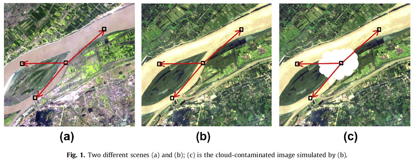
Some notations
- \(I(x, y)\): input image (target image),
- \(R(x, y)\): reconstructed image (imputed image),
- \(L(x, y)=(s_x, s_y)\) : offset map,
-
\(p = (x,y)\): a pixel in the target image,
-
\(p\)' : the pixel of the reference image in the same position as \(p\),
-
\(N\): the spatial 4-connected neighbor system of the images,
-
\(p\)'': a 4-connected neighbor of \(p\) in the target image.
-
\(L(p)=(s_x, s_y)\) means that we copy the pixel at \((x+s_x, y+s_y)\) to the location \((x,y)\).
-
\(\Omega\) is the missing region
A reconstructed pixel \(R(x, y)\) will be derived from \(I(x+s_x, y+s_y)\). Therefore, our goal is to calculate a suitable offset map \(L(x, y)\) for all the pixels in the missing region.
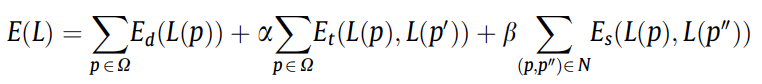
The optimal offset map minimizes the following spatio-temporal MRF energy function:
Spatio-temporal Markov random fields (STMRF) model
- The first term \(E_d\) is a data term. \(E_d\) is 0 if the label is valid (i.e., \(x+s_x, y+s_y)\) is a known pixel, not located at the missing region); otherwise it is \(+\infty\).
-
The second term \(E_t\) is a temporal smoothness term which is used to enforce the offset \(L(p)\) to be similar to the offset \(L(p')\).

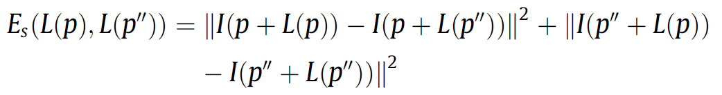
- The third term \(E_s\) is a spatial smoothness term.
This smoothness term takes into account the consistency of the spatial neighbors between the missing region and the remaining region in the target image
The energy function is optimized using multi-label graph cuts
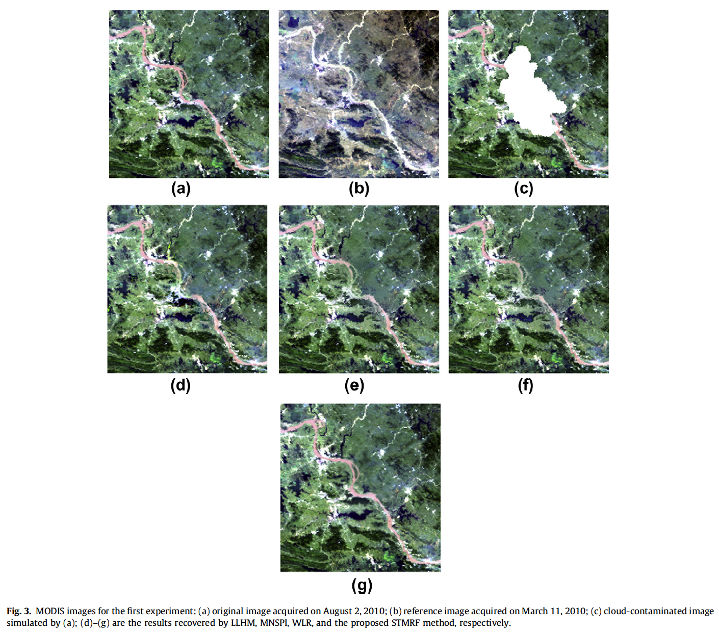
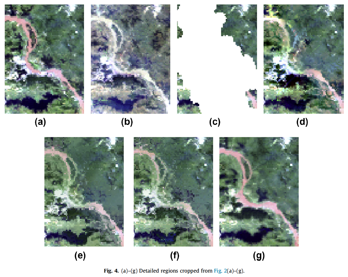
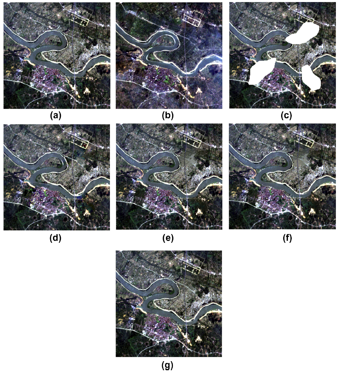
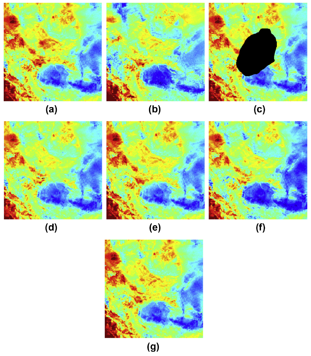
Results on MODIS
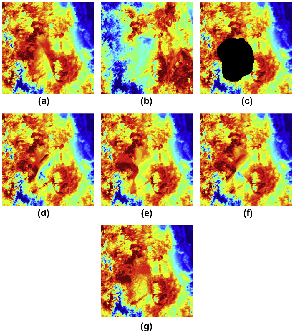
Results on Landsat TM
Results on MODIS LST 1
Results on MODIS LST 2
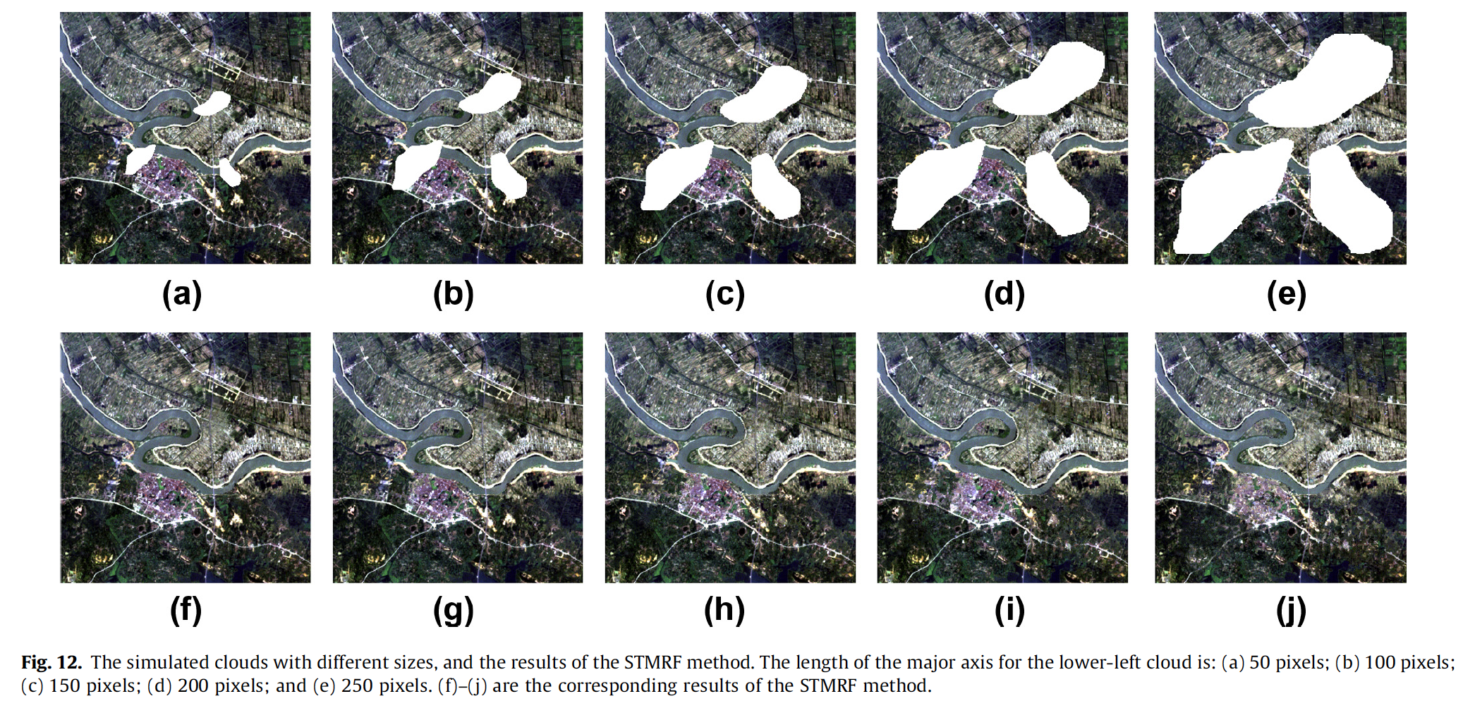
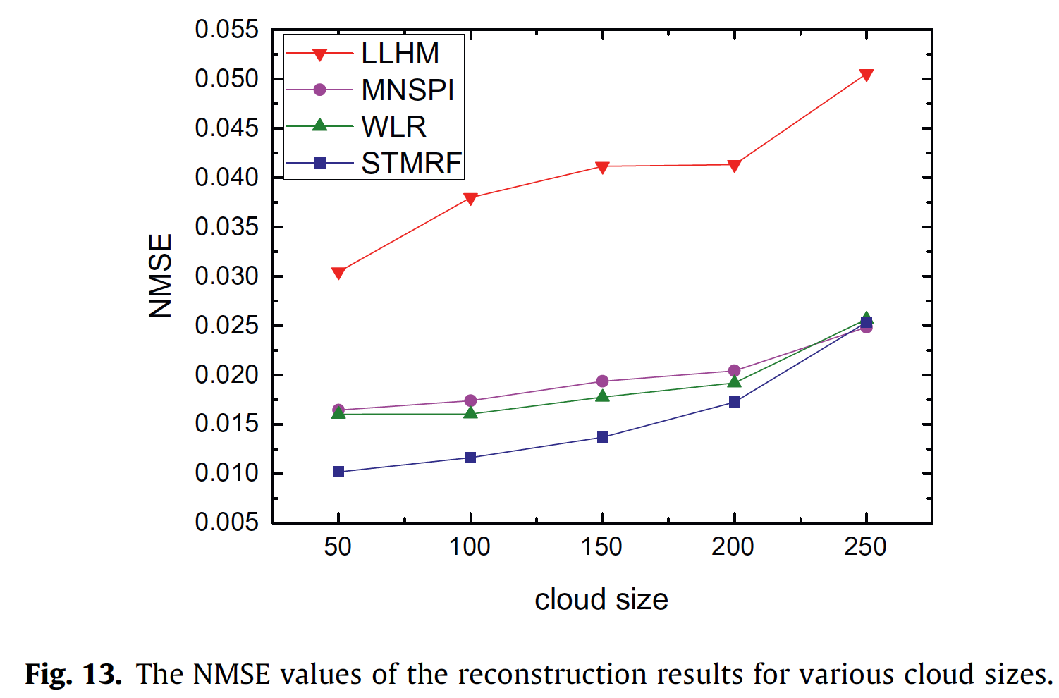
Sensitivity to cloud size
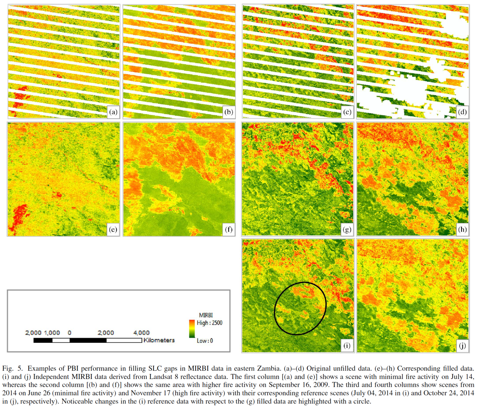
The profile-based interpolator
(PBI)
This paper provide a very nice literature review, but lack of pictures in illustrating the gap filling procedure.
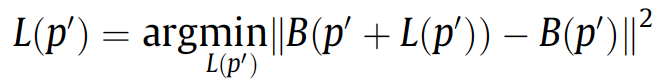
1. Temporal Profile Alignment
The algorithm
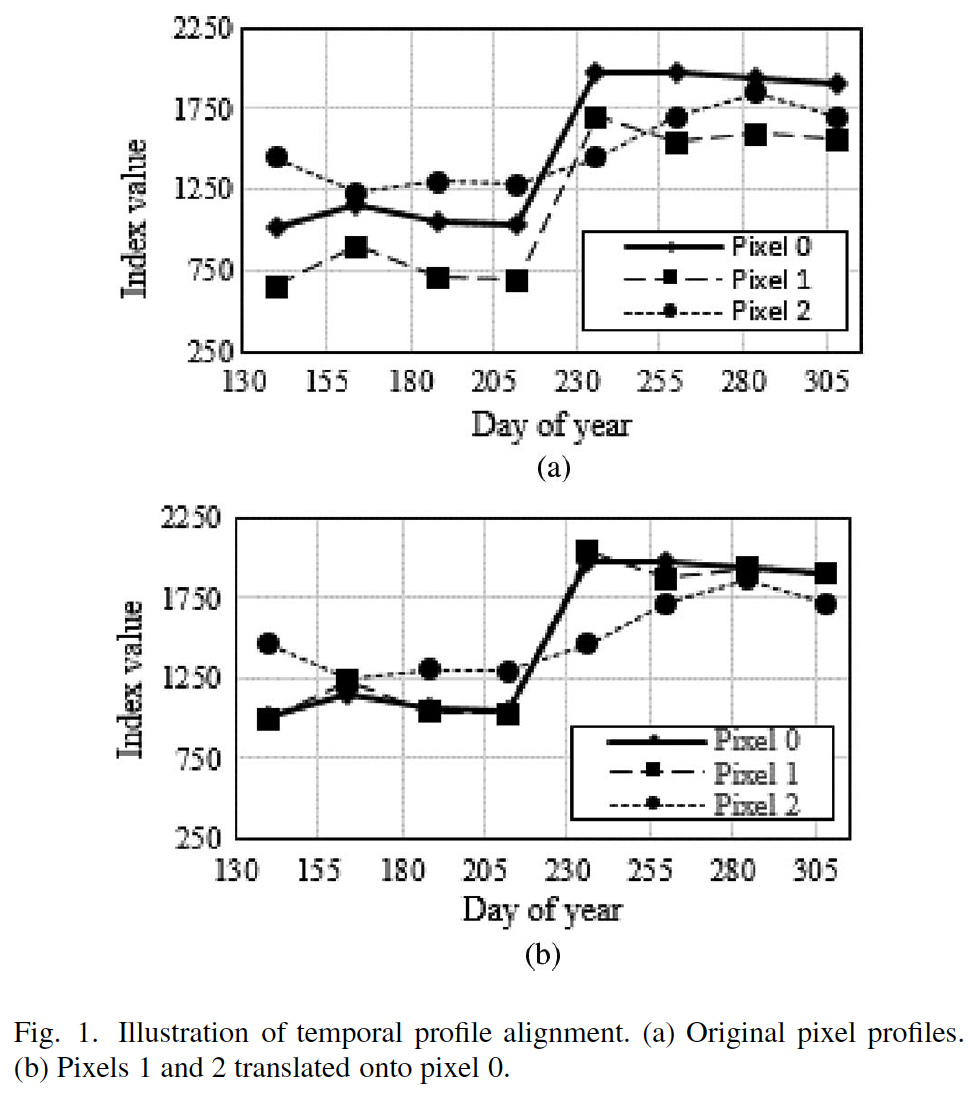
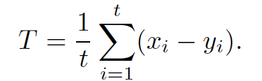
The offset T is estimated by
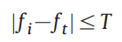
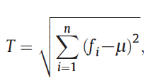
2. Selection of Similar Profiles.
Pixels with similar temporal profiles are selected within a set processing image window based on similarity to the target profile with missing values.
Similarity to the target profile is evaluated using the maximum deviation percent calculated as
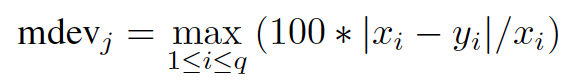
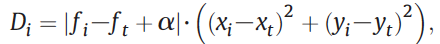
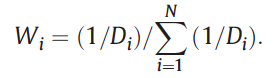
2. Estimating Missing Values.
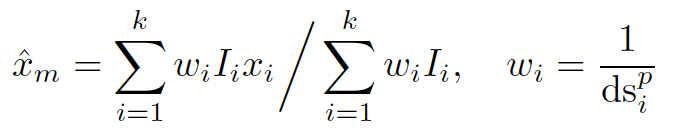
Missing values are estimated by a weighted (inverse distance weight) average of the selected k similar values.
To fill large gaps, if complete profiles exist in the data set, the interpolation process is initialized at pixels near complete data and proceeds inward as in a region-growing algorithm.
The process is iteratively repeated, using existing and estimated data, until all missing pixel values are filled.
Example
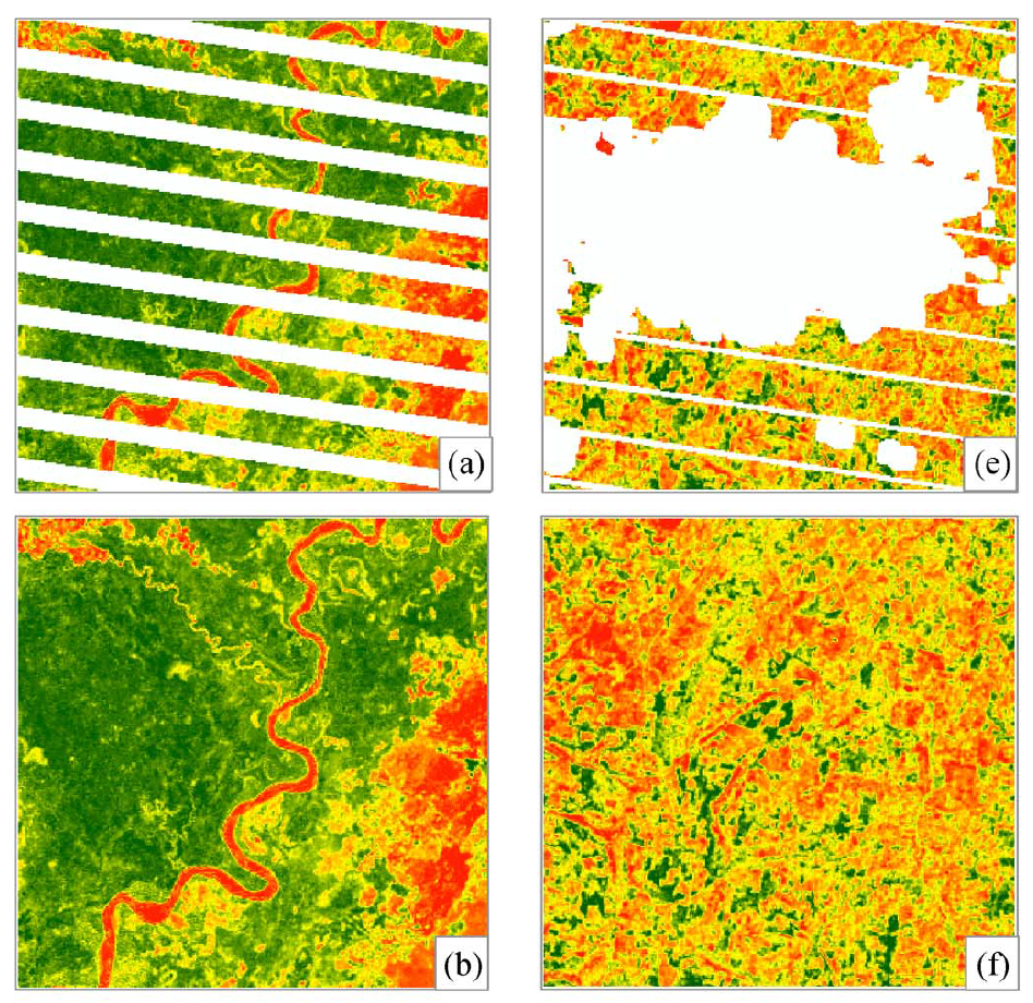
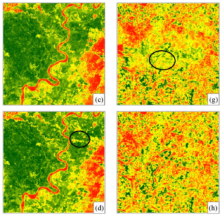
a) e) simulated missing pattern. b) f) original image.
c) d) results using PBI method g) h) results using BPFA method
Tempo-Spectral Angle Model
(TSAM)
Some notations
- \((x, y)\) are the spatial location;
- \(t\) is the temporal number;
- \(\lambda\) is the spectral waveband;
- \(L\) is the original input multitemporal data;
- Each image is composed of \(M\times N\) pixels;
- Each pixel contains \(K\times T\) elements (\(K\) is the number of total spectral bands and \(T\) is the total temporal number;
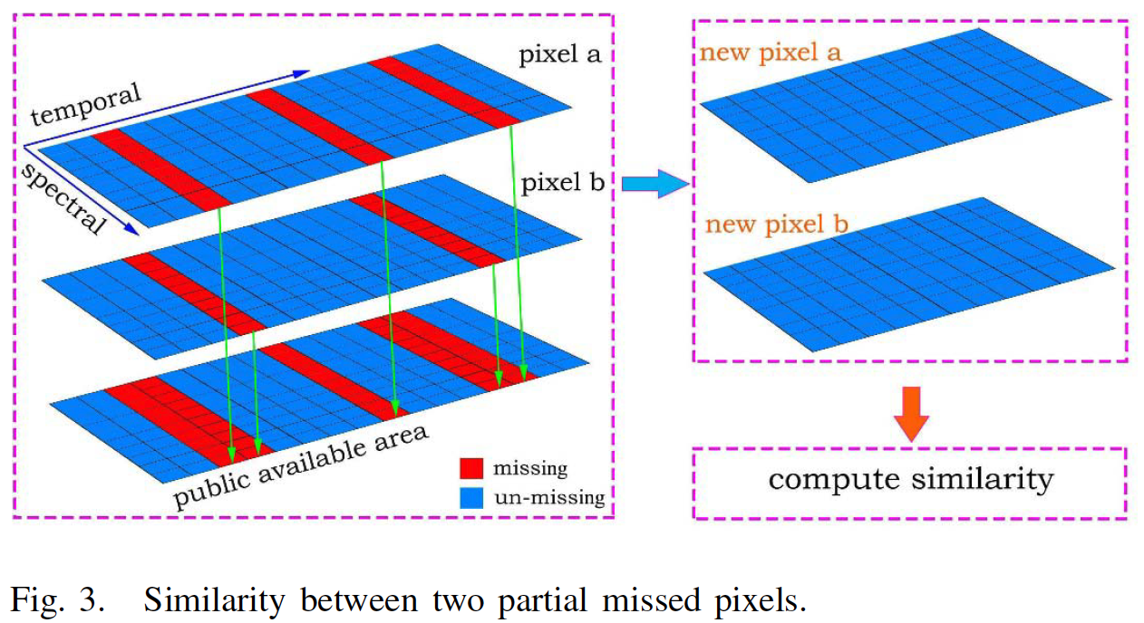
- Denote \(X\) as input pixel and \(Y\) as reference pixel (\K \times T\) matrix;
- \(x_{i,j}\) and \(y_{ij}\) are the elements of \(X\) and \(Y\) located at the \(i\)th row and \(j\)th column.
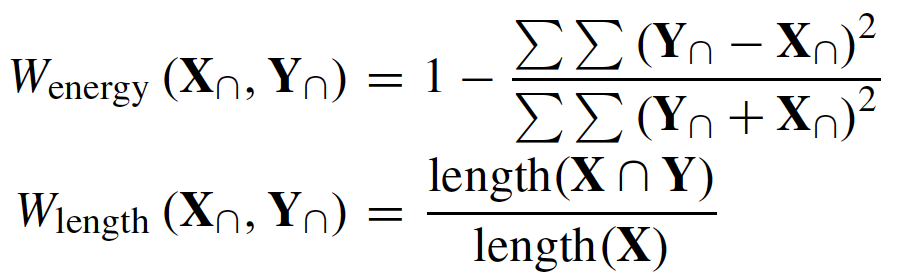
Tempo-Spectral Angle Mapping (TSAM)
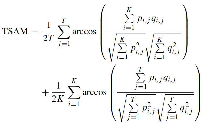
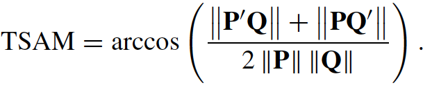
Define TSAM as follows to measure the similarity between two pixels which are described under spectral and temporal dimensions
Algorithm
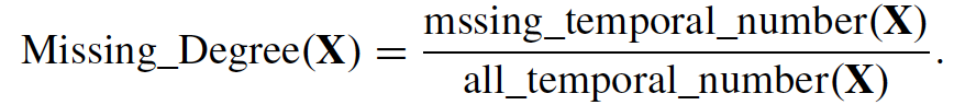
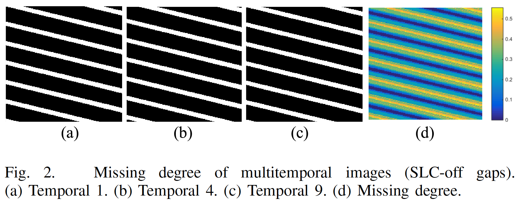
1. Finding the Filling Pixel by using data missing degree. The lower missing degree pixels should be recovered first.
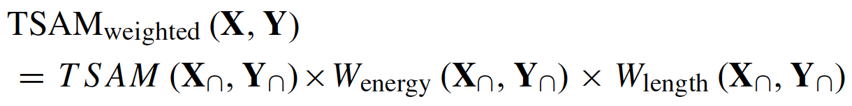
2. Finding the similar pixel based on weighted TSAM.
By taking into account of the total reflected energy and the temporal number, a weighted TSAM is used to find the similar pixel:
3. Filling the partial missing input pixels using similarity replacement.
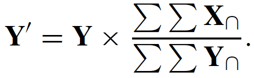
After transform the reference pixel \(Y\) to \(Y'\), the unmissing part in \(Y'\) will be used to replace the correspoinding location of input missing pixel \(X\).
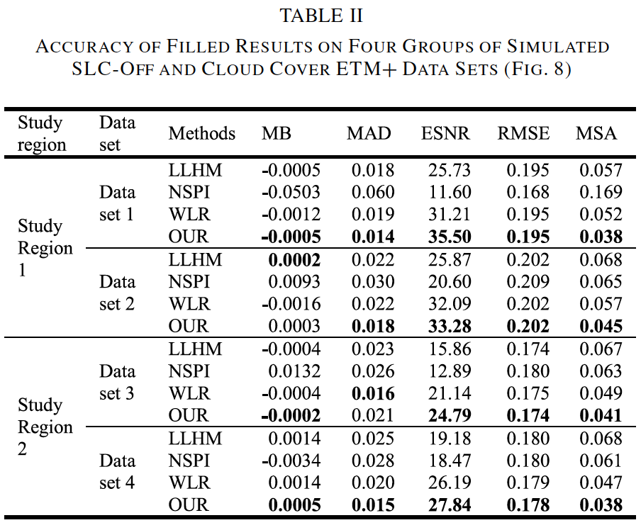
Results
gapfill
By mingsnu
