High-energy radiation from
pulsar-star wind colliding binaries
Víctor Moreno de la Cita
Heidelberg, 6th May 2015
Valentí Bosch-Ramon
Dmitry Khangulyan
We performed a 2D axisymmetric RHD simulation (Paredes-Fortuny et al. 2015) of the pulsar-star wind collision followed by a computation of the evolution of the non-thermal particles and their IC and synchrotron radiation.
Gamma ray binaries as
early type star + compact object.
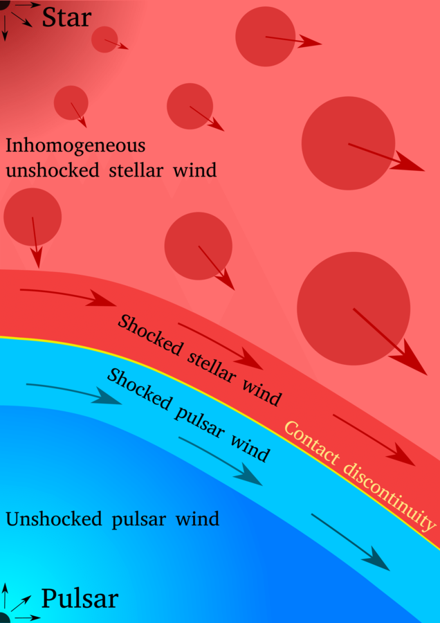
We consider the gamma-ray production in the colliding wind region of binaries with a non-accreting pulsar
We consider an inhomogeneous stellar wind, with a clump placed between the pulsar and the star.
To do so, we first impose an homogeneous wind until we reach a stationary state and then we add a clump of a given size and density.
Our workframe
Paredes-Fortuny et al. 2015
We fix our coordinate system with the y axis in the line connecting the pulsar and the star. The shock is formed where the ram pressures of the two winds are balanced.
Our workframe
T_{\star} = 4\times 10^4 \text{ K}
L_{\star} = 10^{39} \text{erg s}^{-1}
\vec{v}_{wind,\star} = 3000 \text{ km s}^{-1}
\dot{M}_\star = 10^{-7} M_\odot \text{yr}^{-1}
The star is a O type with the following data:
R_c = 1 \text{ or }5 \text{ in units of } a, \text{ with }\,\, a = 8\times 10^{10} \text{ cm}
Clump radius:
Our workframe
The pulsar has a spin-down luminosity of:
And a wind Lorentz factor of:
L_{sd} = 10^{37}\text{ erg s}^{-1}
\Gamma = 5
Giving rise to a pulsar-to-star wind momentum ratio of :
\eta = \dfrac{F_{pw}S_{pw}}{F_{sw}S_{sw}}\approx\dfrac{L_{sd}}{\dot{M}v_{sw}c}\approx 0.2
y_\star = 4.4\times 10^{12} \text{ cm}
y_p = 4\times 10^{11} \text{ cm}
Star
Pulsar
Our workframe
Star
Pulsar
Although the RHD simulation is 2D, we take this information and scramble the different lines around the y axis, giving each line a random azimuthal angle phi, so the result is more similar to the 3D real scenario.
Going into details. hidrodynamic setup.
Dealing with fluid mixing
The fluid is divided in 40 lines with 200 cells each, describing an axisymmetric 2D space of:
r\in[0,2.4\times10^{12}\text{ cm}]
However, not every line contains shocked material, so we can ignore some. Also, given that the two winds can mix through the fluid lines, we have had to cut the lines at a certain point.
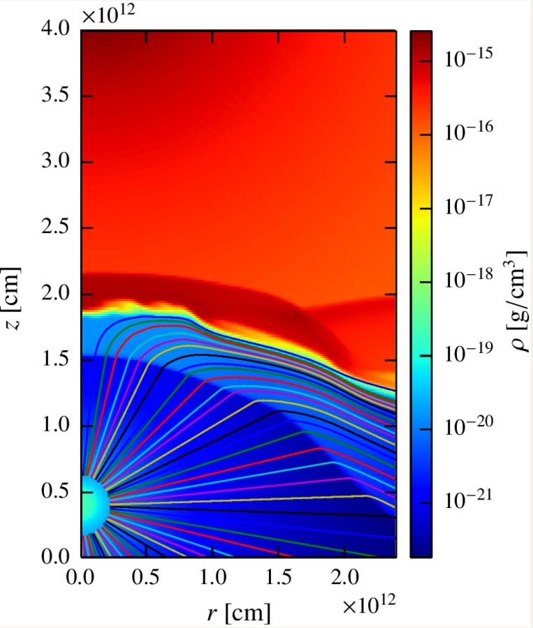
y\in[0,4\times10^{12}\text{ cm}]
Going into details. Physical assumptions i.
Prescription for acceleration in strong shocks (Drury 1983)
t_{gain} = t_{loss}
t_{loss} = \min
\{
t_{sync}=\dfrac{1}{a_sB^2E}
t_{diff} = \dfrac{R^2}{2D}, \,\,\,D=k\cdot r_g\cdot c/3
t_{gain} = \tilde\eta \dfrac{E}{qBc}
\tilde\eta=2\pi(c/v)^2
with
We inject non-thermal particles when a shock takes place:
Internal energy goes up
and
fluid velocity goes down
Where and how do we inject non-thermal particles
Going into details. Physical assumptions ii.
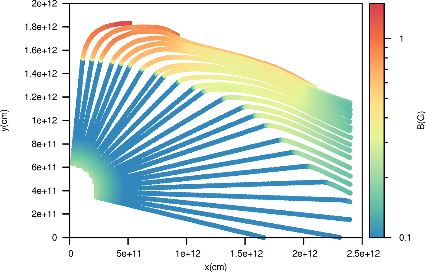
Magnetic field perpendicular to the fluid line
B_0^\prime = \Gamma_0^{-1}\sqrt{\eta_B \times 8\pi e_0}
e_0 = \Gamma_0^2\rho_0h_0c^2 - \Gamma_0\rho_0 c^2 -p_0
B_k^\prime = B_0^\prime \Big( \dfrac{\rho_k v_0\Gamma_0}{\rho_0 v_k \Gamma_k}\Big)^{1/2}
\eta_B = 10^{-4}, 1
Definition of the magnetic field at the beginning of the line:
Evolution of the B field in the different cells k:
(Low, high magnetic field)
Free energy density
Fraction of total energy that goes to magnetic energy
Going into details. some notes on the code.
- We let the particles evolve until they reach a steady state so we can consider the medium stationary, in other words, every loss time (e.g. synchrotron) or cell-crossing time is much shorter than the dynamical time on large scales.
- All the computation is done in the (relativistic) frame of the fluid, so every relevant quantity has to be transformed, including the angles between fluid, gamma photons and target photons velocities.
- The section evolution is computed imposing conservation of energy in the fluid frame.
S = S_0\dfrac{\Gamma_0^2\rho_0h_0v_0}{\Gamma^2\rho hv}
Going into details. Structure of the shock.


Paredes-Fortuny et al. 2015
Going into details. Magnetic field.
No clump
Small clump
Big clump
As proposed by Bosch-Ramon 2013
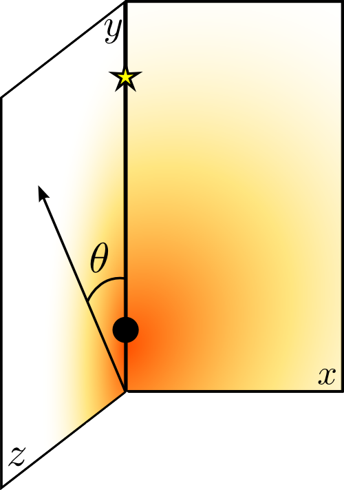
Going into details. Observer angle.
Star
Pulsar
To avoid eclipses, we do not simulate the most extreme cases:
\theta = 0,\,\theta=180^\circ
Instead, we take just three angles: 45º for the case of the observer closer to the star, 135º for the one closer to the pulsar and 90º, when the observer is placed in the z axis.
The observer will be placed in the z-y plane forming an angle theta with the vertical axis.
Results. Low magnetic field, no clump.
Very similar sync. emission, the IC depends stronger on the viewing angle.
The absorption due to pair production depends on the position of the observer and the extent of the IC source.
Results. Low magnetic field, 90 degrees.
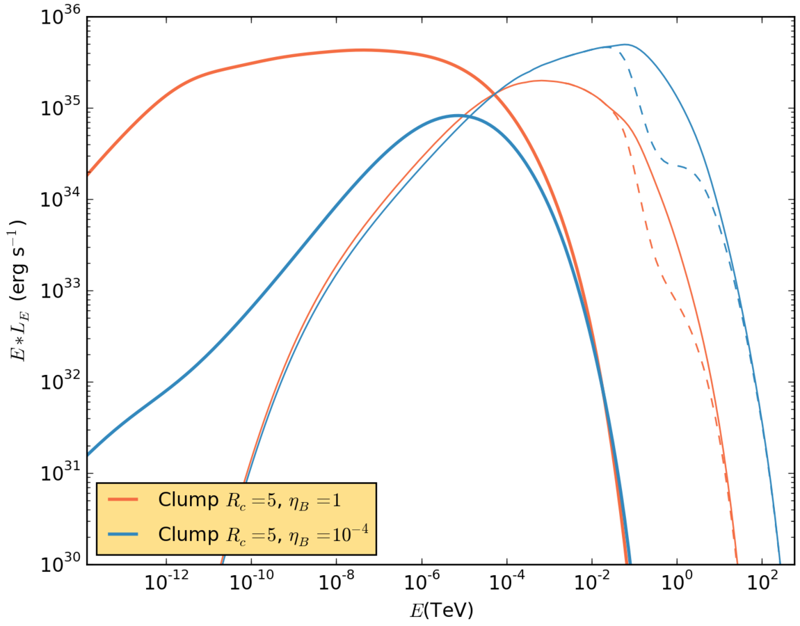
Small clumps do not seem to change importantly the emission of the homogeneous wind. However, if the clump is big enough, an increase on both synchrotron and IC emission is expected.
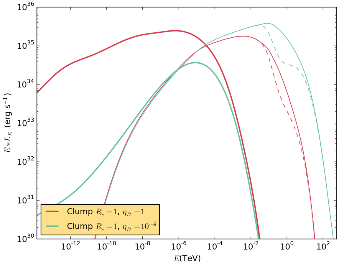
Results. small clump with different B fields.
With a B field 100 times stronger, the IC radiation becomes weaker and presents a cutoff at lower energy.
The synchrotron emisson becames much more important, specially at low energies.
Results. big clump with different B fields.
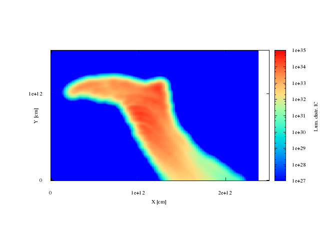
Maps. IC radiation, big clump.
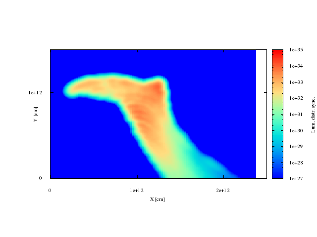
Maps. synchrotron radiation, Big clump.
Discussion. Conclusions and future work.
The next step could be to get a more realistic 3D scenario computing a larger number of lines to make the scramble.
With this method we should be able to:
- Explore different scenarios of academical interest
- Try to explain the gamma-ray emission of some sources such as PSR B1259-63 or LS I +61 303.
Thank You.
Backup slide. Fixing the line ending.
Given that the two winds can mix through the fluid lines, we have had to cut the lines at a certain point. To do so, we can impose that the amount of material that crosses the section do not get larger than a certain threshold:
\text{if: } S\rho v\Gamma > 2\times S_0\rho_0v_0\,\rightarrow\, \text{end of the line}
if: SρvΓ>2×S0ρ0v0→end of the line
Backup slide. Injected Luminosity.
The injected non-thermal particles have a lumisosity given by:
L_{inj} = \chi \times \dfrac{L_T}{ \Gamma^2} \dfrac{v_{rel}}{v}
Linj=χ×Γ2LTvvrel
L_T= U_T\Gamma^2vS
LT=UTΓ2vS
With the pre-factor varying between 0 and 1 and the total luminosity being:
heidelberg2015
By otnoesmusica
heidelberg2015
High-energy radiation from pulsar-star wind colliding binaries


