Star-jet interactions in AGN and their
high-energy emission
Санкт-Петербург, 9th September 2016
V. M. DE LA CITA

Getting started: motivations
Active galactic nuclei (AGN) jets can interact with every kind or stellar populations. Also, AGN activity has been proved to be closely related with starbursts (mentioned before in this meeting in the talk by A. Eckart), so the occurrence of interactions between the jet and the stellar population is expected to be frequent .
Dynamical effects
non-thermal emission
Star-jet interactions: a tale of two winds
- 70's: Blandford & König 79 propose stars/clouds can form shocks inside AGN jets
- 80's: Several authors (Frölik et al. 89, Rees 87, Penston 88) explore the possibility of the BLR being the interactive cloud.
- 90's: Analytical (Komissarov 94) and numerical (Bowman et al. 96) studies of the dynamical impact of stars on AGN jets.
- 00's: Hubbard & Blackman 06, Perucho et al. 14 - disruption of the jet by stars.
Impact on the jet dynamics
Komissarov 94
Star-jet interactions: a tale of two winds
- 90's: Bednarek & Protheroe 97 first studied the possibility
- S. XXI: Several authors have explored the blazar, non-blazar, transient and persistent high energy emission (Barkov, Khangulyan, Bosch-Ramón, Araudo)
- Even observational evidence could exist (Hardcastle et al. 2003, Müller et al. 2014)
Gamma-ray emission
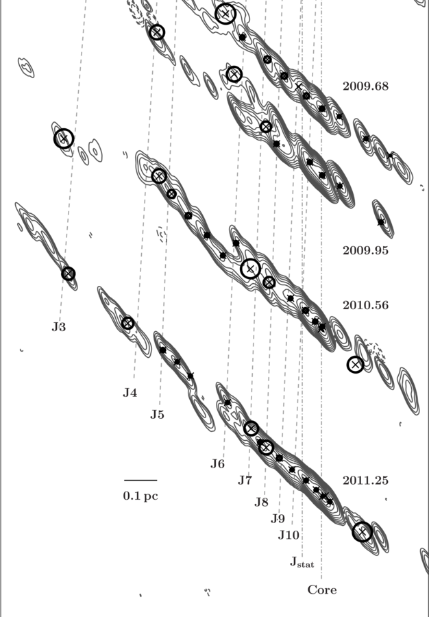
Inner parsec of Centaurus A
Müller, C. et al. 2014
Bednarek & Protheroe 1997; Barkov et al. 2010, 2012; Khangulyan et al. 2013;
Bosch-Ramon et al. 2012; Araudo et al. 2010,2013; Bosch-Ramon 2015;
Bednarek & Banasinski 2015, this work.
physical scenario
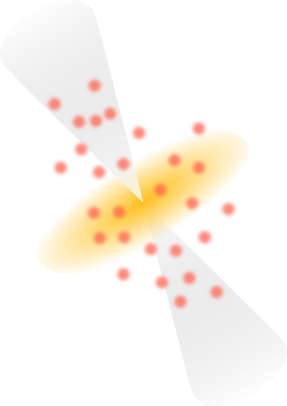
The impact of stars and its atmospheres on AGN jets has been studied previously by other authors.
A number of problems must be addressed: the type of star populations, the impact of the stars in the jet dynamics...
We perform hydrodinamic simulations ot the regions close to the star, and then we compute its non-thermal emission.
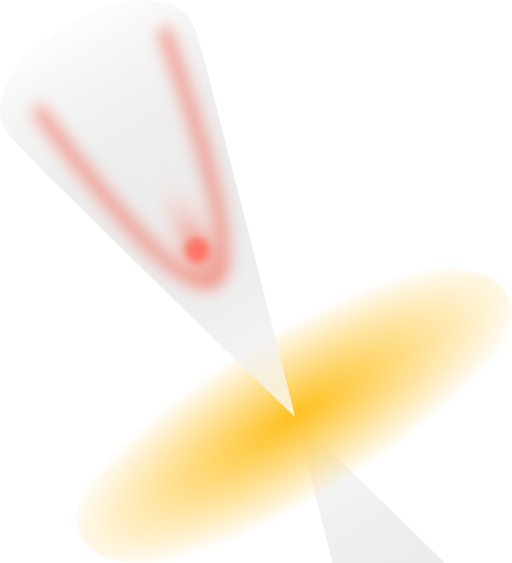
physical scenario. A single star
Inner parsec of Centaurus A
Müller, C. et al. 2014
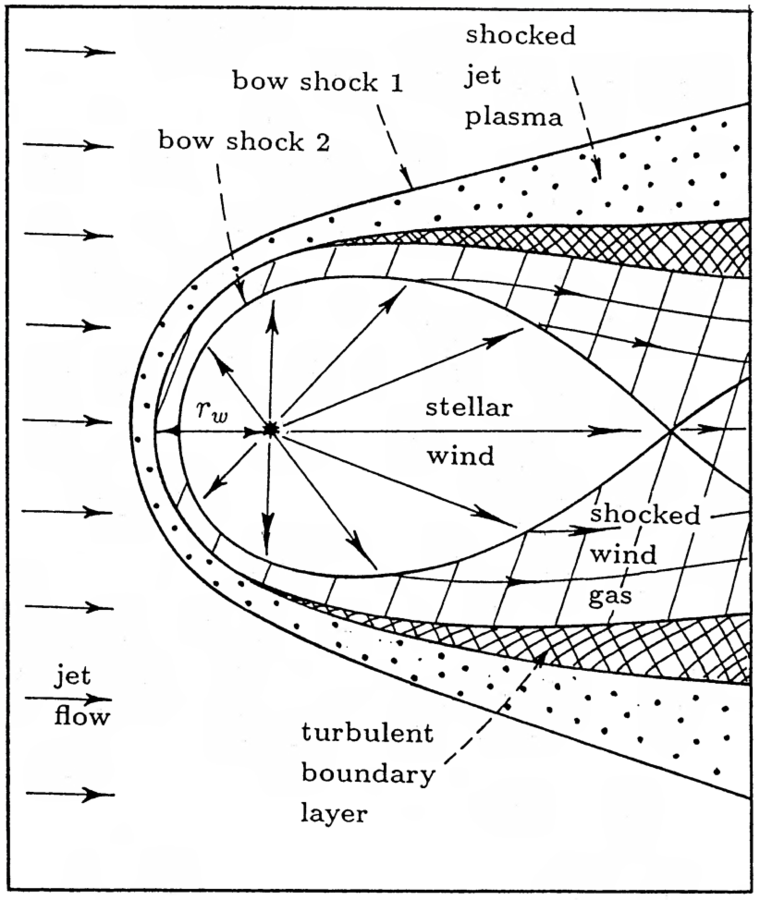
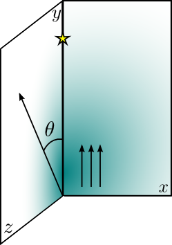
We fix our coordinate system with the y axis in the line connecting the base of the jet and the star. The shock is formed where the ram pressures of the two winds are balanced.
Our workframe
\vec{v}_\text{stellar wind} = 2000 \text{ km s}^{-1}
\dot{M}_\star = 10^{-9} M_\odot \text{yr}^{-1}
The stellar wind is uniform with the thrust of a high mass star with moderate mass-loss rate (the corresponding thrust also typical for red giants) with the following data:
The jet has a luminosity of:
and a wind Lorentz factor of:
L_\text{jet} \sim 10^{44}\text{ erg s}^{-1}
\Gamma = 10
for a 1 pc radius
Going into details. hidrodynamic setup.
The fluid is divided in 77 lines with 200 cells each, describing an axisymmetric 2D space of:
r\in[0,2\times10^{15}\text{ cm}]
y\in[0,1.5\times10^{15}\text{ cm}]
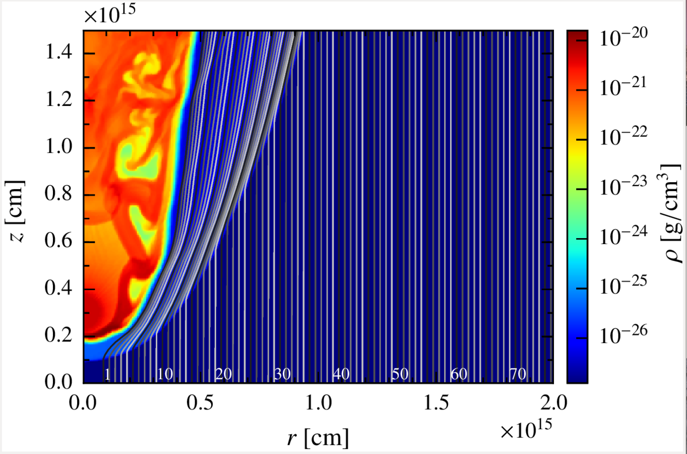
y_\star = 3\times 10^{14} \text{ cm}
Although the RHD simulation is 2D, we take this information and scramble the different lines around the y axis, giving each cell a random azimuthal angle phi, so the result is more similar to the 3D real scenario from the observer viewpoint.
Going into details. 3d emitter.

Going into details. Physical assumptions.
Magnetic field perpendicular to the fluid line
\dfrac{B_0^{\prime 2}}{4\pi} = \chi_B (\rho_0h_0cv)
\chi_B = 10^{-4}, 0.1
Definition of the magnetic field at the beginning of the line:
(Low, high magnetic field)
Fraction of matter energy flux that goes to magnetic energy (Poynting flux)
Photon field:
T_{\star} = 3\times 10^3 \text{ K}
L_{\star} = 3\times 10^{36} \text{erg s}^{-1}
injection of non-thermal particles in the fluid:
A fraction of the generated internal energy per second in a given cell (at the shocks) is transferred to non-thermal particles.
\chi = 0.1
Going into details. some notes on the code.
- We let the particles evolve until they reach a steady state so we can consider the medium stationary, in other words, every loss time (e.g. synchrotron) or cell-crossing time is much shorter than the dynamical time on large scales.
- All the particle evolution and radiation computations are done in the (relativistic) frame of the fluid, so every relevant quantity has to be transformed, including the angles between fluid, gamma photons and target photons velocities.
- Once we have the electron distribution, we compute the inverse Compton (IC) and synchrotron radiation, taking into account Doppler boosting.
\delta = 1/\Gamma(1-\beta\cos{\theta_\text{obs}})
\epsilon L(\epsilon)= \delta^4\epsilon'L(\epsilon')
where
Going into details. Observer angle.
To sample a wide range of possibilities, we take four angles: 0º (with the jet bulk velocity pointing at the observer), 45º, 90º (when the observer is placed on the z axis) and 135º.
The observer will be placed beyond the star forming an angle theta with the vertical axis.
Star
Jet thrust
\theta = 0^\circ, 45^\circ, 90^\circ, 135^\circ
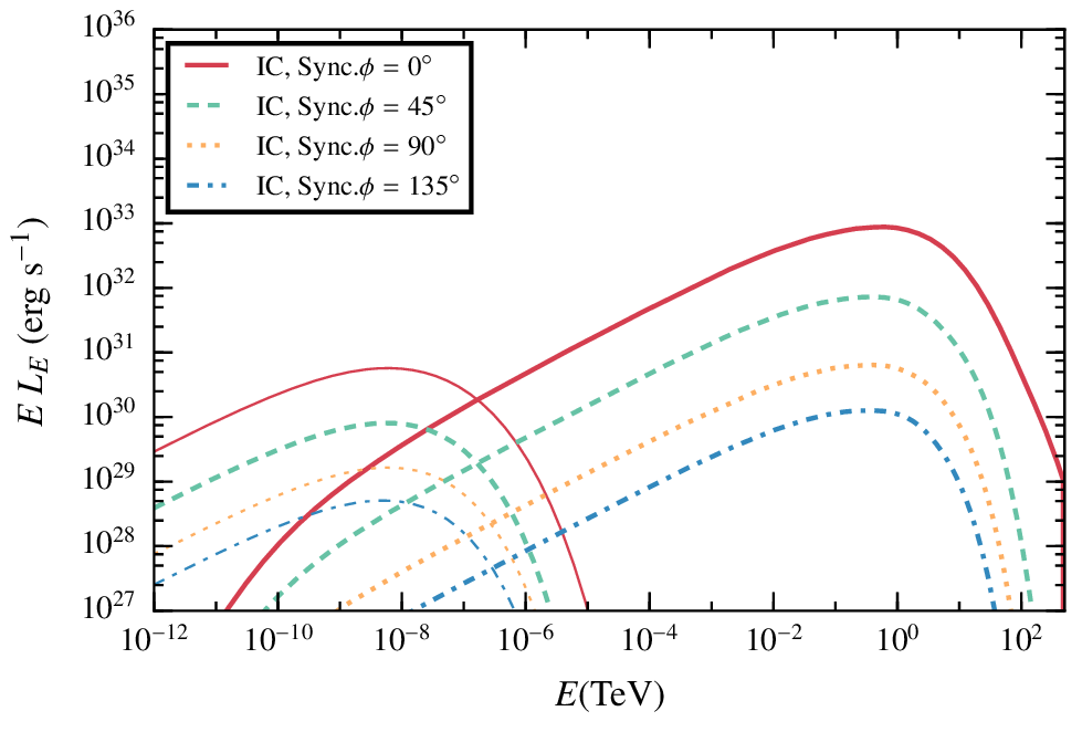
Results. Low magnetic field, steady state.
In the case of a low magnetic field, the IC radiation dominates the spectrum.
The difference between the four angles come from the doppler boosting, more important for smaller angles given that most of the cells have a strong y- component of the velocity
\chi_B = 10^{-4}
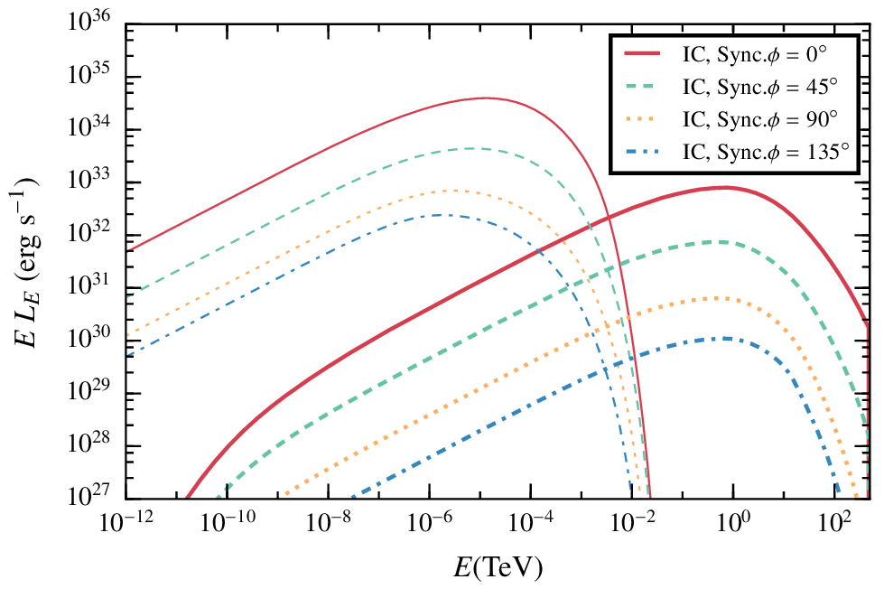
Results. high magnetic field, steady state.
In this case the synchrotron emission dominates the spectrum, whereas the IC is very similar.
\chi_B = 0.1
Synchrotron emission can play an important role at GeV energies even with not-so-extreme magnetic fields.
Results. perturbed state.
In some cases, the instabilities can eventually lead to a perturbed state of the shock, increasing the effective area of the emitter.
Results. perturbed state with with different B fields and angles
When the instabilities lead to a perturbed state of the shock, a transient increment of the synchrotron luminosity is expected.
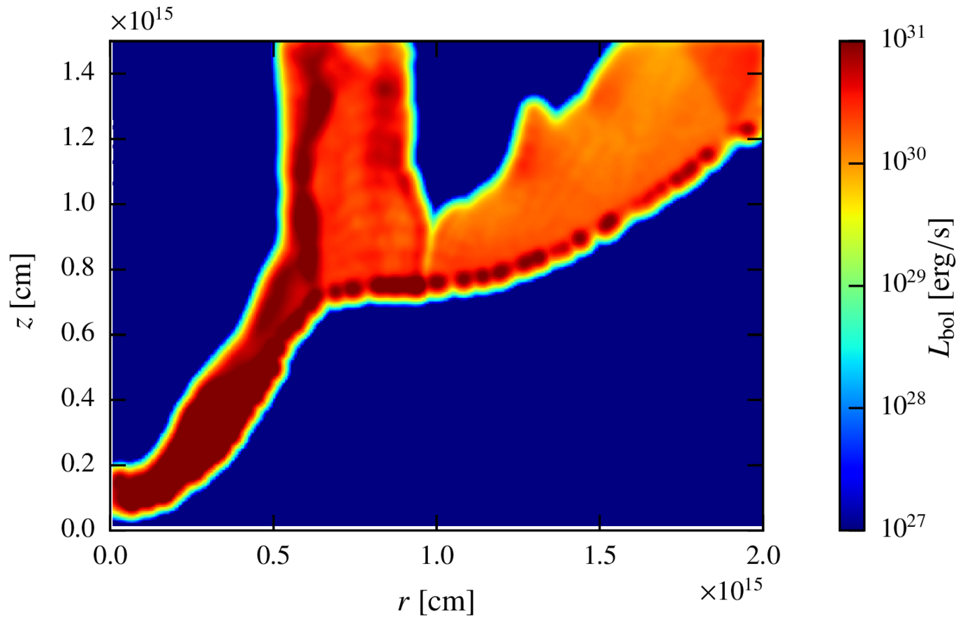
Maps. Steady state.
Inverse compton
The total observer luminosity in this case is:
r < r_{CD}
\chi_B = 10^{-4},\,\,\theta = 0^\circ
Whereas the luminosity of the region with
L_{IC}=5 \times 10^{34} \text{erg s}^{-1}
is ~100 times smaller, so the effective size of the emitter is much larger than the CD region.
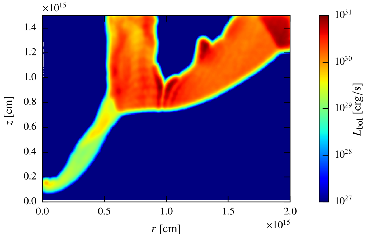
Maps. Steady state.
synchrotron
The total observer luminosity in this case is:
For the synchrotron, the emission is even more equally distributed through the shock, because it does not depend on the external photon field.
L_{sync}=2.5 \times 10^{32} \text{erg s}^{-1}
\chi_B = 10^{-4},\,\,\theta = 0^\circ
Maps. perturbed state.
Inverse compton
synchrotron
\chi_B = 10^{-4},\,\,\theta = 0^\circ
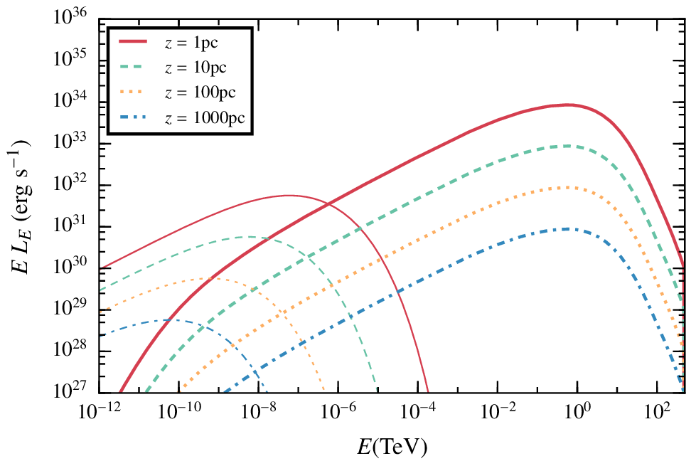
Discussion. Scalability of the results
\chi_B = 10^{-4},\,\,\theta = 0^\circ
Our hydrodinamical simulation places the star at a jet height of z = 10pc, but the results can be easily scaled with z.
L_\text{rad}\propto 1/z
If the losses are dominated by escape:
Discussion. Conclusions.
- The effective radius of the emitter is much bigger than the contact discotinuity radius.
- Emission levels strongly depend on the viewer angle due to Doppler boosting.
- The non-thermal luminosity for a single star points towards potentially detectable luminosities for typical populations crossing AGN jets, according to Bosch-Ramón 15 estimates.
V. M. de la Cita, V. Bosch-Ramon, X. Paredes-Fortuny, D. Khangulyan and M. Perucho, 2016, A&A, 591, A15
Thank You.
Going into details. Physical assumptions i.
We follow a prescription for particle acceleration in strong shocks. The acceleration timescale goes like ~1/v² as proposed in previous works (e.g. Drury 1983)
We inject non-thermal particles when a shock takes place:
Internal energy goes up
and
fluid velocity goes down
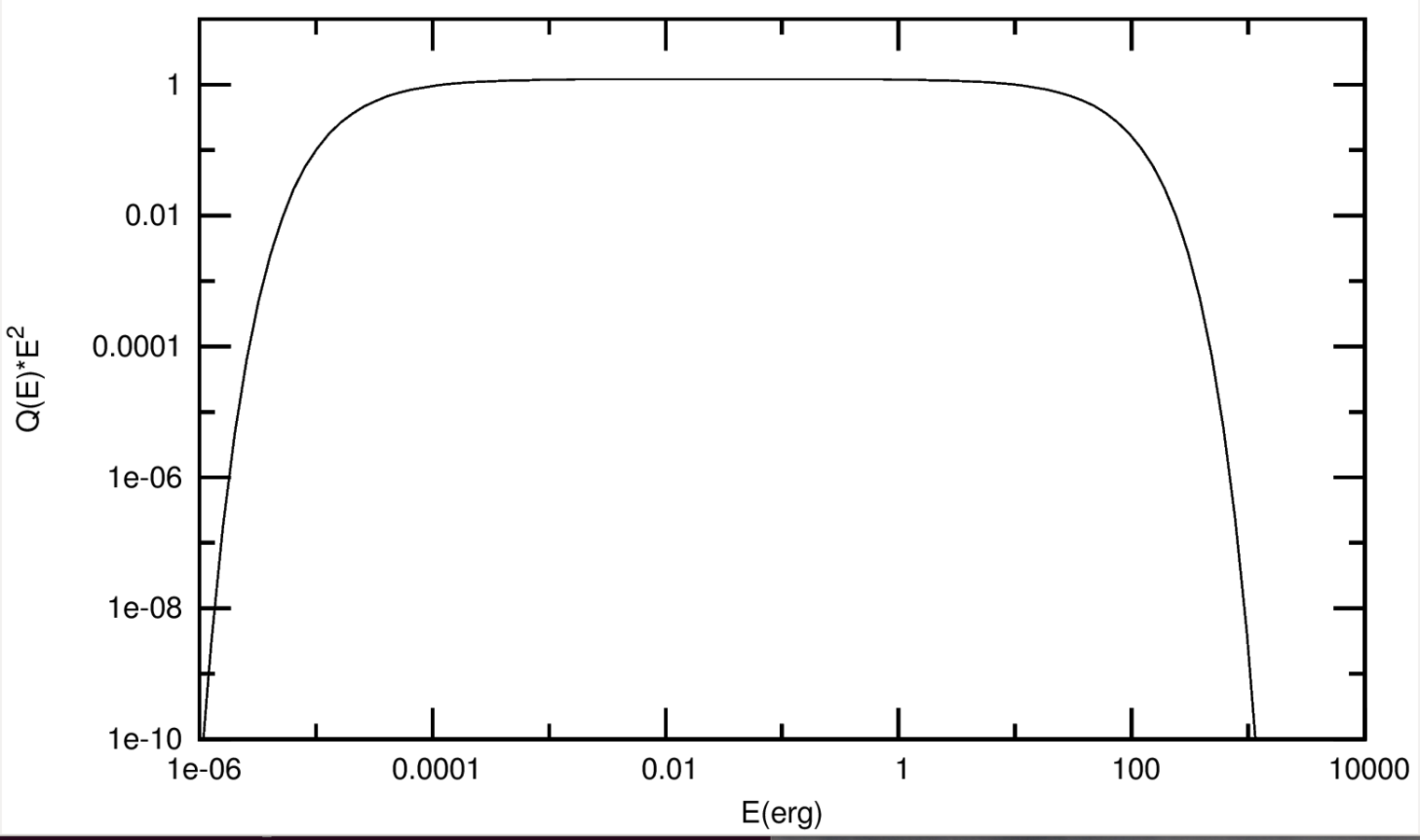
Where and how do we inject non-thermal particles
Q(E) \propto E^{-2} \times (e^{-E_{min}/E})^5 \times e^{-E/E_{max}}
t'_\text{acc}=\eta E'qB'c, \text{with}
\eta = 2\pi (c/v)^2
Backup slide. Fixing the line ending.
Given that the two winds can mix through the fluid lines, we have had to cut the lines at a certain point. To do so, we can impose that the amount of material that crosses the section do not get larger than a certain threshold:
\text{if: } S\rho v\Gamma > 2\times S_0\rho_0v_0\,\rightarrow\, \text{end of the line}
Backup slide. Injected Luminosity.
The injected non-thermal particles have a lumisosity given by a fraction of the generated internal energy per second in the cell.
L_{inj} = \chi_{NT} \times \dot{U}'_k =
With the pre-factor varying between 0 and 1 and the +/- subindexes refering to the right/left boundaries, respectively.
= \chi_{NT} v_k\Gamma_k^2\times \left(S_+\Gamma_+^2h_+\rho_+c^2\left(1 +\dfrac{v_+^2}{c^2}\right) - S_-\Gamma_-^2h_-\rho_-c^2\left(1 +\dfrac{v_-^2}{c^2}\right)\right)
APCS 2016
By otnoesmusica
APCS 2016
Star-jet interactions in AGN and their high-energy emission


