Coupling fluid-dynamics and non-thermal processes to study sources of high-energy emission
28th April 2017
Víctor Moreno DE LA CITA

Supervisors: Valentí Bosch-Ramon, Dmitry Khangulyan
Outline
-
sources with relativistic outflows moving in rich environments
-
Methods: coupling hydrodynamics and NT calculation
-
Three relevant cases of study:
-
star-jet interactions in active galactic nuclei
-
pulsar wind interacting with a clumpy stellar wind
-
clumpy wind-jet interacions in high-mass microquasars
-
Concluding remarks
2/59
sources with relativistic outflows
moving in rich environments
AGN GRB Binaries with pulsar Microquasars
Extragalactic sources galactic sources
Astrophysical sources with relativistic outflows are good candidates to accelerate particles to the highest energies. The environments of these sources can play an important role in both galactic and extragalactic sources (e.g. Bordas et al. 2011) so we have explored the interaction of the outflow with the medium as the main site of particle acceleration.
Among the sources with relativistic outflows that present gamma-ray emission we have:
3/59
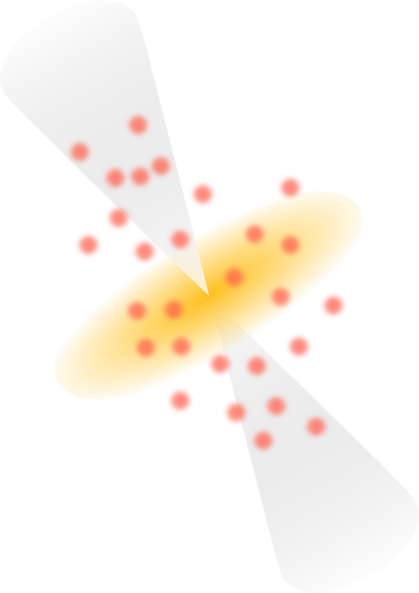
Active galactic nuclei

Credit: Seeds (1997)
Acceleration of particles may take place at several sites inside a galaxy containing an AGN, such as the corona, the jet itself or at its termination shock.
AGN GRB Binaries with pulsar Microquasars
sources with relativistic outflows
moving in rich environments
4/59
Complex environments
The surroundings of an AGN are complex environments by nature, given they are placed in the centre of galaxies. A large number of stars and gas clouds are crossing the relativistic outflows of the jets constantly.
sources with relativistic outflows
moving in rich environments
AGN GRB Binaries with pulsar Microquasars
5/59
- 70's: Blandford & König 79 propose stars/clouds can form shocks inside AGN jets
- 90's: Analytical (Komissarov 94) and numerical (Bowman et al. 96) studies of the dynamical impact of stars on AGN jets.
- 00's: Hubbard & Blackman 06, Perucho et al. 14 - disruption of the jet by stars.
Impact of the stars on the jet dynamics
Komissarov 1994
AGN GRB Binaries with pulsar Microquasars
sources with relativistic outflows
moving in rich environments
6/59
- 90's: Bednarek & Protheroe 97 studied the possibility
- S. XXI: Several authors have explored the blazar, non-blazar, transient and persistent high energy emission (Barkov, Khangulyan, Bosch-Ramon, Araudo, Bednarek,Banasinski)
- Even observational evidence could exist (Hardcastle et al. 2003, Müller et al. 2014, Wykes et al. 2015)
Gamma-ray from the star-jet interaction
Radio image of the inner parsec of Centaurus A (Müller et al. 2014)AGN GRB Binaries with pulsar Microquasars
sources with relativistic outflows
moving in rich environments
7/59
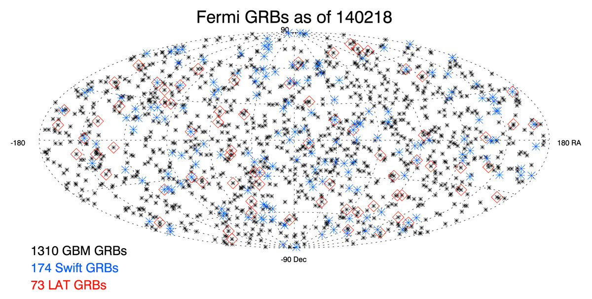
GAMMA-ray bursts
Credit:
Gruber et al. (2014)  Kienlin et al. (2014)
Not covered in this thesis
Transient, fast emission associated with the merger of compact objects or the collapse of massive stars and of extragalactic origin.
AGN GRB Binaries with pulsar Microquasars
sources with relativistic outflows
moving in rich environments
8/59
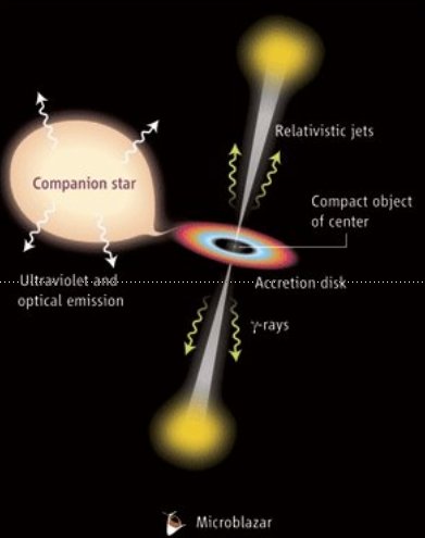
high-mass binaries with pulsars and microquasars
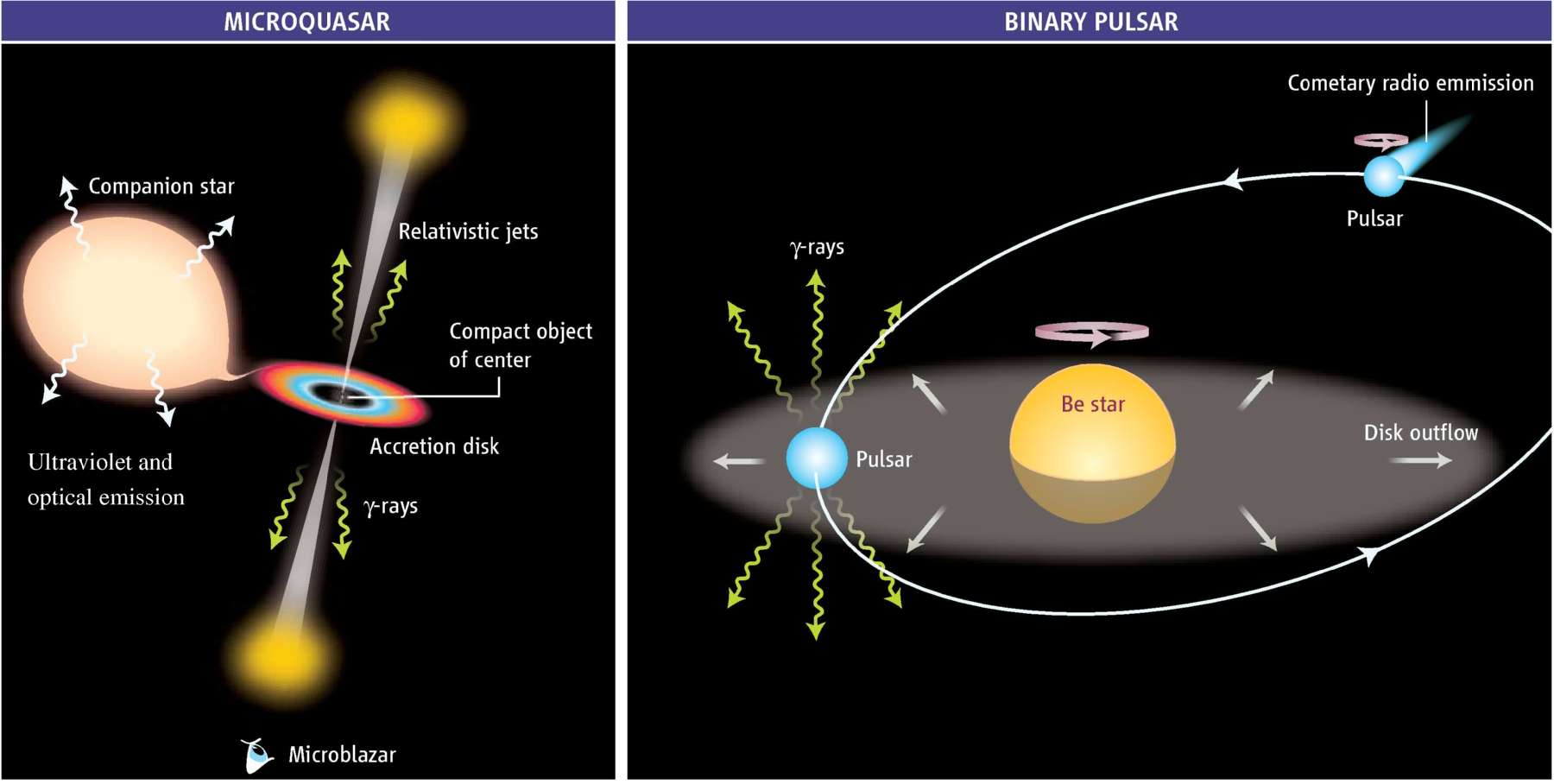
Credit: Mirabel (2006)
High-mass stars with a non-accreting pulsar orbiting around may accelerate particles in the interaction between the star's and the pulsar's wind and produce NT radiation.
Example: PSR B1259-63
Microquasars are composed by a compact object and star, but in this case the compact object accretes material from the star. This may lead to the formation of two jets, observable from radio to X-rays and, in some cases, gamma-rays. If the star is massive they are called high-mass microquasars.
Examples: Cygnus X-1 and Cygnus X-3
AGN GRB Binaries with pulsar Microquasars
sources with relativistic outflows
moving in rich environments
9/59
Complex environments
F. Mirabel
The winds the massive stars (O, B type) are expected to be strongly inhomogeneous, presenting overdensities (Owocki & Cohen 2006, Moffat 2008).
These overdensities are called clumps and may interact with the (relativistic) outflow from the compact object: the wind of a pulsar or the jets in a microquasar.
AGN GRB Binaries with pulsar Microquasars
sources with relativistic outflows
moving in rich environments
10/59
Non-thermal processes
Non-thermal
emission
The most powerful sources and most energetic events are dominated by non-thermal processes: hard to observe, hard to model and impossible to reproduce in a laboratory (produced by very energetic -accelerated- particles)
11/59
Non-thermal processes
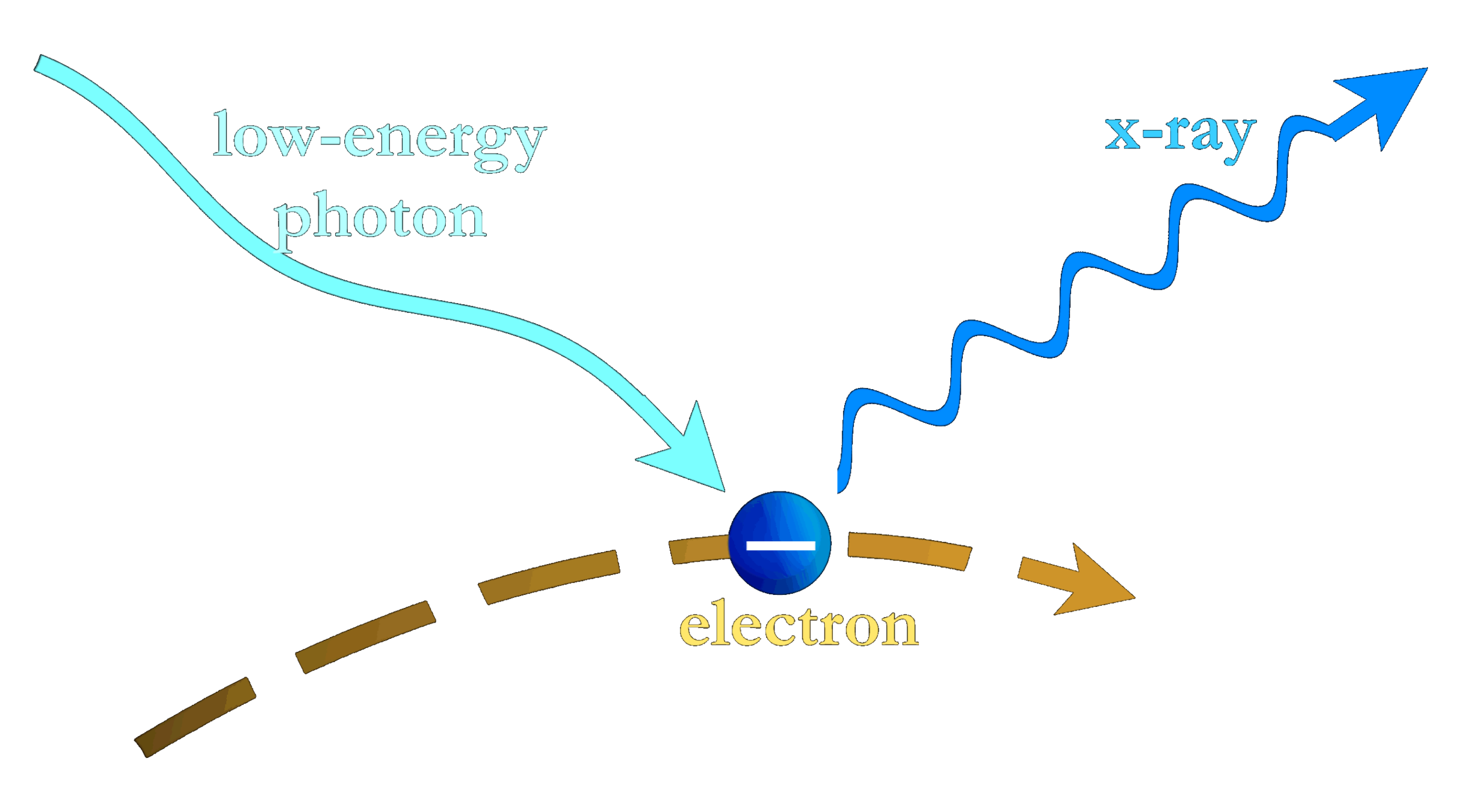
Inverse compton (IC)
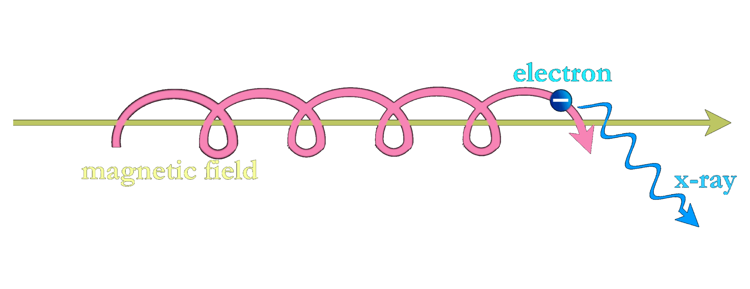
Synchrotron
An energetic electron collides with a photon, increasing its energy up to x-rays or gamma-rays.
Accelerated electrons, spiraling around a magnetic field, can emit high energy photons.
Credit: Chandra
Bremsstrahlung, hadronic processes, etc
In the systems we have studied, these two processes are the most important (see e.g. Bosch-Ramon & Khangulyan 2009)
12/59
Coupling Hydrodynamics And NT computation
Absorption by pair creation
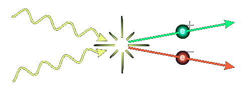
Positron
Electron
Gamma photon
Low-energy photon
Given the high energy of the gamma-ray photons, they can create a electron-positron pair if they interact with the surrounding (stellar) photon field. This results in an effective absorption of gamma photons.
13/59
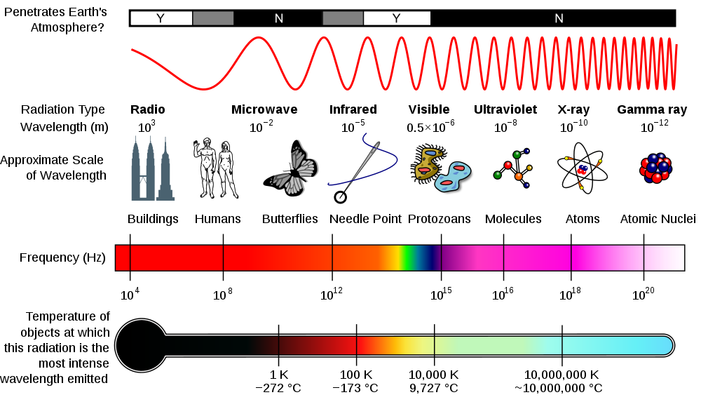
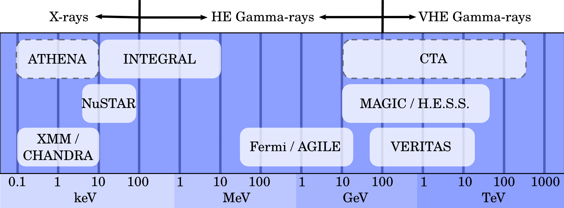
gamma-ray astronomy
Gamma rays allow us to study non-thermal (NT) processes of emission in astronomical sources, given that at these energies there is no contamination of thermal radiation.
Space satellites like Fermi or AGILE and ground-based Cherenkov array telescopes like MAGIC, H.E.S.S., VERITAS or HAWC are the current observational tools in gamma rays.
14/59
Outline
-
star-jet interactions in active galactic nuclei
-
pulsar wind interacting with a clumpy stellar wind
-
clumpy wind-jet interacions in high-mass microquasars
-
Concluding remarks
-
sources with relativistic outflows moving in rich environments
-
Methods: coupling hydrodynamics and NT calculation
-
Three relevant cases of study:
15/59
Coupling Hydrodynamics And NT computation
Outline
- Perform relativistic hydrodynamic simulations of the system. In our case, 2D axisymmetric simulations.
- Extract the streamlines of the simulated fluid.
- Compute the injection of NT particles, assuming a given acceleration efficiency.
- Let the particles evolve inside the fluid, until a steady-state is reached.
- Compute the NT emission. We focused on the most efficient channels in our systems: inverse Compton (IC) and synchrotron emission. We also take into account the absorption due to pair production.
- Plot SEDs and maps of the results.
This part was done by our collaborators
16/59
Coupling Hydrodynamics And NT computation
Hydrodynamic setup and streamline calculation
We perform relativistic hydrodynamic simulations in 2D taking advantage of the axisymmetry of our systems.
In this simulations the magnetic field was not included.
Later we define a set of fluid elements at the bottom of our grid and we draw the trajectories they follow (streamlines). Each streamline is also divided in 200 cells.
17/59
Coupling Hydrodynamics And NT computation
Magnetic fields in the systems
\dfrac{B_0^{\prime 2}}{4\pi} = \chi_B (\rho_0hcv)
\chi_B
Fraction of matter energy flux that goes to magnetic energy (Poynting flux)
To set the magnetic field at the beginning of the streamline we assume that a fraction of matter energy flux goes into magnetic energy:
Assuming an ideal plasma we have applied the frozen in theorem (Alfvén 1942). The magnetic field in our cells would be perpendicular to the fluid and proportional to the section of the streamlines.
B_k^\prime = B_0^\prime \Big( \dfrac{\rho_k v_0\Gamma_0}{\rho_0 v_k \Gamma_k}\Big)^{1/2}
Evolution of the B field in the different cells k:
18/59
Coupling Hydrodynamics And NT computation
Internal energy goes up
and
fluid velocity goes down
Particle acceleration in shocks
Q(E) \propto E^{-2} \times (e^{-E_{min}/E})^5 \times e^{-E/E_{max}}
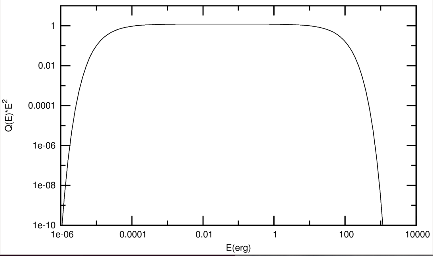
A fraction of the generated internal energy per second in a given cell is transferred to NT particles. This fraction is a free parameter in our simulations, given the little knowledge we have about it.
The acceleration of particles takes place inside the shocks formed in the fluid. We inject non-thermal particles in the code when a shock takes place:
19/59
Coupling Hydrodynamics And NT computation
Particle evolution and NT radiation
- We let the particles evolve until they reach a steady state so we can consider the medium stationary, in other words, every loss time (e.g. synchrotron) or cell-crossing time is much shorter than the dynamical time on large scales.
- Once we have the electron distribution, we compute the inverse Compton (IC) and synchrotron radiation, including the absorption if it is significant.
- All the particle evolution and radiation computations are done in the (relativistic) frame of the fluid, so every relevant quantity has to be transformed, including the angles between fluid, gamma photons and target photons velocities. Also the Doppler boosting has to be taken into account:
\delta = 1/\Gamma(1-\beta\cos{\theta_\text{obs}})
\epsilon L(\epsilon)= \delta^4\epsilon'L(\epsilon')
where
20/59
Coupling Hydrodynamics And NT computation
21/59
Outline
-
star-jet interactions in active galactic nuclei
-
pulsar wind interacting with a clumpy stellar wind
-
clumpy wind-jet interacions in high-mass microquasars
-
Concluding remarks
-
sources with relativistic outflows moving in rich environments
-
Methods: coupling hydrodynamics and NT calculation
-
Three relevant cases of study:
22/59
Bednarek & Protheroe 1997; Barkov et al. 2010, 2012; Khangulyan et al. 2013;
Bosch-Ramon et al. 2012; Araudo et al. 2010,2013; Bosch-Ramon 2015;
Bednarek & Banasinski 2015, this work.
physical scenario
The impact of stars and its atmospheres on AGN jets has been studied previously by other authors.
A number of problems must be addressed: the type of star populations, the impact of the stars in the jet dynamics...
We perform hydrodinamic simulations ot the regions close to the star, and then we compute its non-thermal emission.
23/59
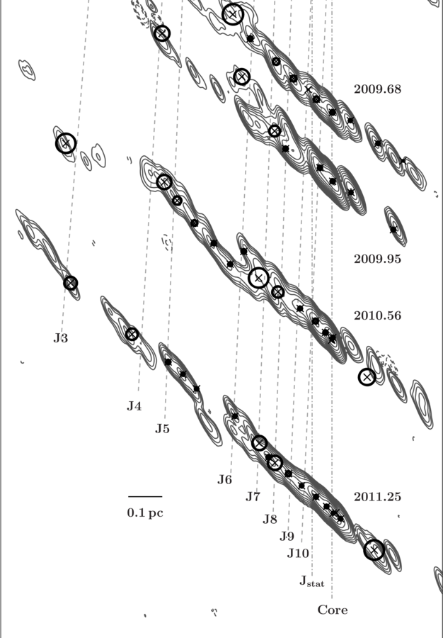
physical scenario. A single star
Inner parsec of Centaurus A
Müller, C. et al. 2014
10 pc
24/59
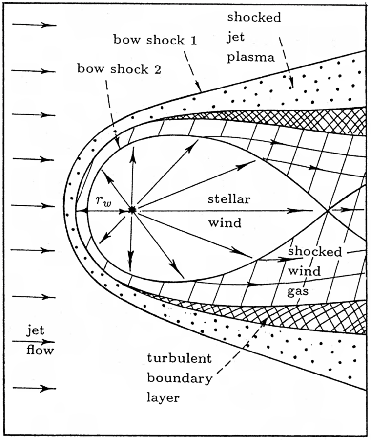
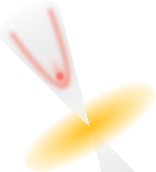
We fix our coordinate system with the z axis in the line connecting the base of the jet and the star. The shock is formed where the ram pressures of the two winds are balanced.
Our workframe
\vec{v}_\text{stellar wind} = 2000 \text{ km s}^{-1}
\dot{M}_\star = 10^{-9} M_\odot \text{yr}^{-1}
The stellar wind is uniform with the thrust of a high mass star with moderate mass-loss rate (the corresponding thrust also typical for red giants) with the following data:
The jet has a luminosity of:
and a Lorentz factor of:
L_\text{jet} \sim 10^{44}\text{ erg s}^{-1}
\Gamma = 10
for a 1 pc radius
25/59
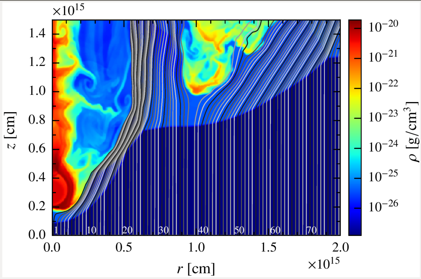
Going into details. hidrodynamic setup.
The fluid is divided in 77 lines with 200 cells each, describing an axisymmetric 2D space of:
r\in[0,2\times10^{15}\text{ cm}]
z\in[0,1.5\times10^{15}\text{ cm}]
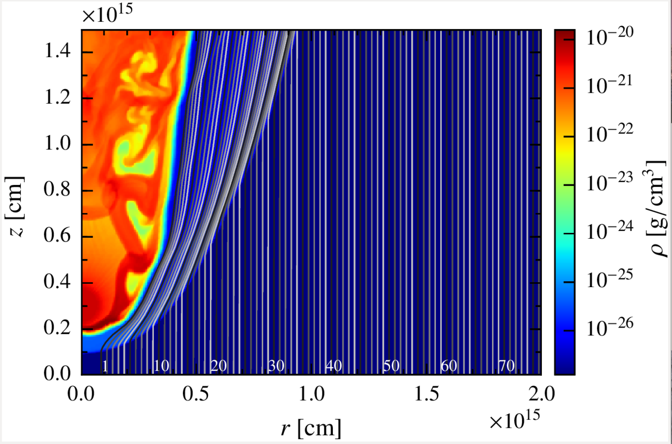
z_\star = 3\times 10^{14} \text{ cm}
26/59
Going into details. Physical assumptions.
Magnetic field:
\dfrac{B_0^{\prime 2}}{4\pi} = \chi_B (\rho_0hcv)
\chi_B = 10^{-4}, 0.1
Definition of the magnetic field at the beginning of the line:
(Low, high magnetic field)
Fraction of matter energy flux that goes to magnetic energy (Poynting flux)
Photon field:
T_{\star} = 3\times 10^3 \text{ K}
L_{\star} = 3\times 10^{36} \text{erg s}^{-1}
27/59
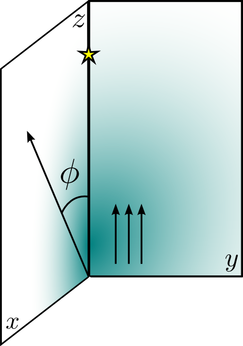
Going into details. Observer angle.
To sample a wide range of possibilities, we take four angles: 0º (with the jet bulk velocity pointing at the observer), 45º and 90º (when the observer is placed on the z axis).
The observer will be placed beyond the star forming an angle phi with the vertical axis.
Star
Jet thrust
\phi = 0^\circ, 45^\circ, 90^\circ
28/59
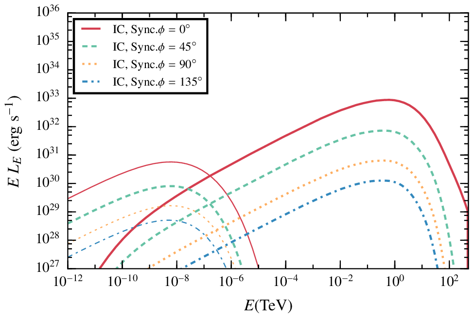
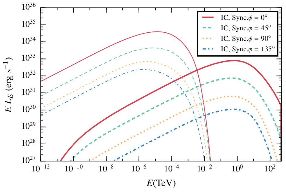
Results. Low magnetic field, steady state.
In the case of a low magnetic field, the IC radiation dominates the spectrum.
The difference between the four angles come from the doppler boosting, more important for smaller angles given that most of the cells have a strong z- component of the velocity
\chi_B = 10^{-4}
29/59
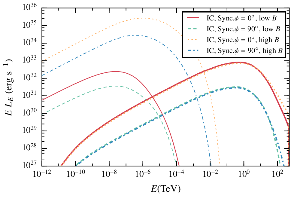
Results. high magnetic field, steady state.
In this case the synchrotron emission dominates the spectrum, whereas the IC is very similar.
\chi_B = 0.1
Synchrotron emission can play an important role at GeV energies even with not-so-extreme magnetic fields.
30/59
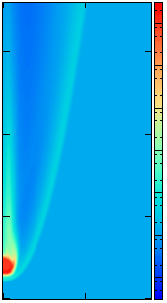
Results. perturbed state.
In some cases, the instabilities can eventually lead to a perturbed state of the shock, increasing the effective area of the emitter.
31/59
Results. perturbed state with with different B fields and angles
When the instabilities lead to a perturbed state of the shock, a transient increment of the synchrotron luminosity is expected.
32/59
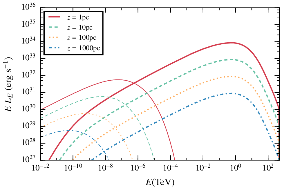
Discussion. Scalability of the results
\chi_B = 10^{-4},\,\,\theta = 0^\circ
Our hydrodinamical simulation places the star at a jet height of z = 10pc, but the results can be easily scaled with z.
L_\text{rad}\propto 1/z
If the losses are dominated by escape:
33/59
AGN jet - star interactions. Conclusions.
- The effective radius of the emitter is much bigger than the contact discotinuity radius.
- Emission levels strongly depend on the viewer angle due to Doppler boosting.
- The non-thermal luminosity for a single star points towards potentially detectable luminosities for typical populations crossing AGN jets, according to Bosch-Ramón 2015 estimates.
- A recent work (Vieyro et al. 2017) suggest that this may be the case in the galaxy 3C 273.
V. M. de la Cita, V. Bosch-Ramon, X. Paredes-Fortuny, D. Khangulyan and M. Perucho, 2016, A&A, 591, A15
34/59
Outline
-
star-jet interactions in active galactic nuclei
-
pulsar wind interacting with a clumpy stellar wind
-
clumpy wind-jet interacions in high-mass microquasars
-
Concluding remarks
-
sources with relativistic outflows moving in rich environments
-
Methods: coupling hydrodynamics and NT calculation
-
Three relevant cases of study:
35/59
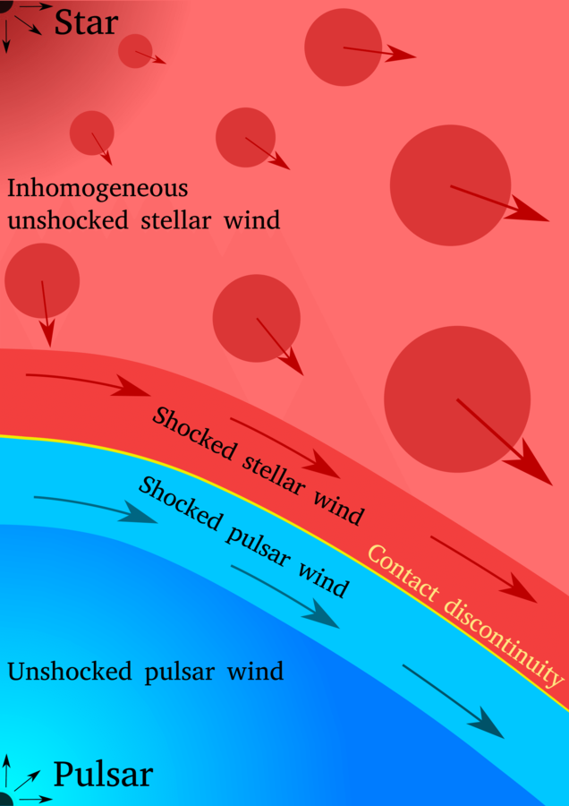
We consider a binary system consisting on a massive star (O type) and a pulsar with a relativistic wind.
Massive stars present strong inhomogeneities in their winds, or clumps (Owocki & Cohen 2006, Moffat 2008). This clumps can affect the interaction of the two winds (Pittard 2007), altering the position of shocks.
Gamma-ray binaries: Early-type star + pulsar
Paredes-Fortuny et al. 2015
36/59
Going into details. hidrodynamic setup.
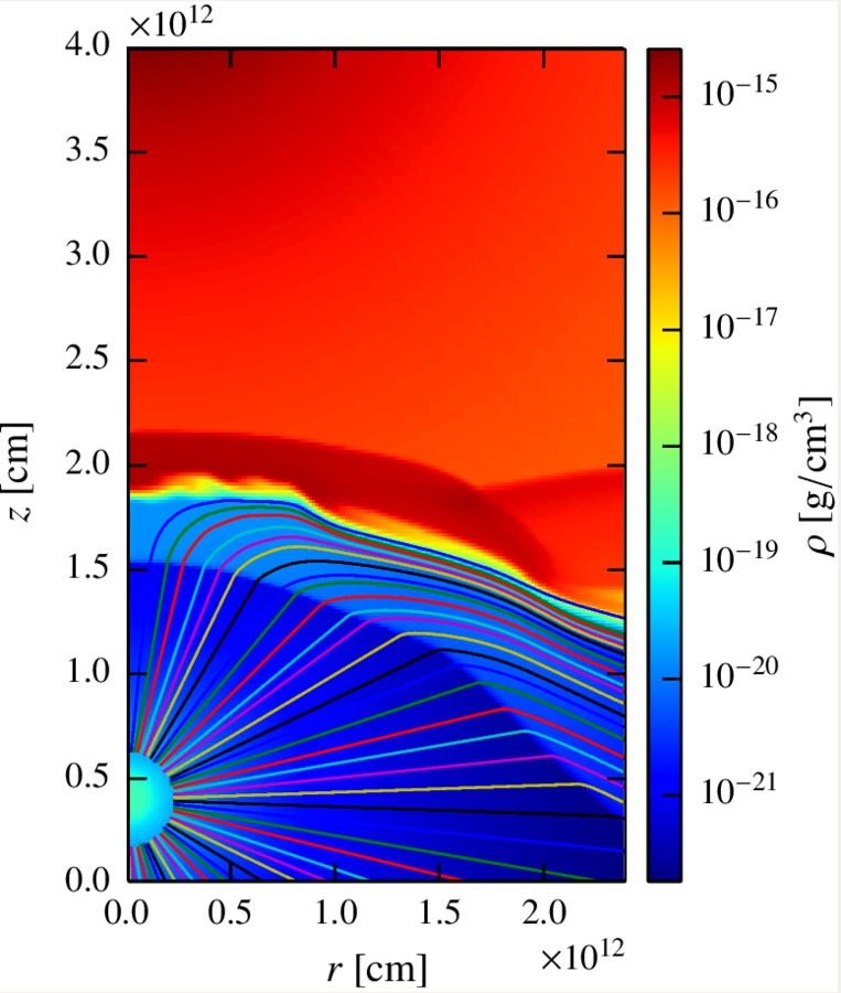
We consider a single clump-wind interaction, with the clump placed between the pulsar and the star.
T_{\star} = 4\times 10^4 \text{ K}
L_{\star} = 10^{39} \text{erg s}^{-1}
\vec{v}_{wind,\star} = 3000 \text{ km s}^{-1}
\dot{M}_\star = 10^{-7} M_\odot \text{yr}^{-1}
R_c = 1 \text{ or }5 \text{ in units of } a,
Clump:
Star:
\text{ with }\,\, a = 8\times 10^{10} \text{ cm}
Pulsar:
L_{sd} = 10^{37}\text{ erg s}^{-1}
\Gamma = 5
z_p = 4\times 10^{11} \text{ cm}
z_\star = 4.4\times 10^{12} \text{ cm}
37/59
Going into details. Structure of the shock.


Paredes-Fortuny et al. 2015
38/59
Going into details. Physical assumptions.
Magnetic field:
\dfrac{B_0^{\prime 2}}{4\pi} = \chi_B (\rho_0hcv)
\chi_B = 10^{-3}, 0.1
Definition of the magnetic field at the beginning of the line:
(Low, high magnetic field)
Fraction of matter energy flux that goes to magnetic energy (Poynting flux)
Photon field:
T_{\star} = 4\times 10^4 \text{ K}
L_{\star} = 10^{39} \text{erg s}^{-1}
39/59
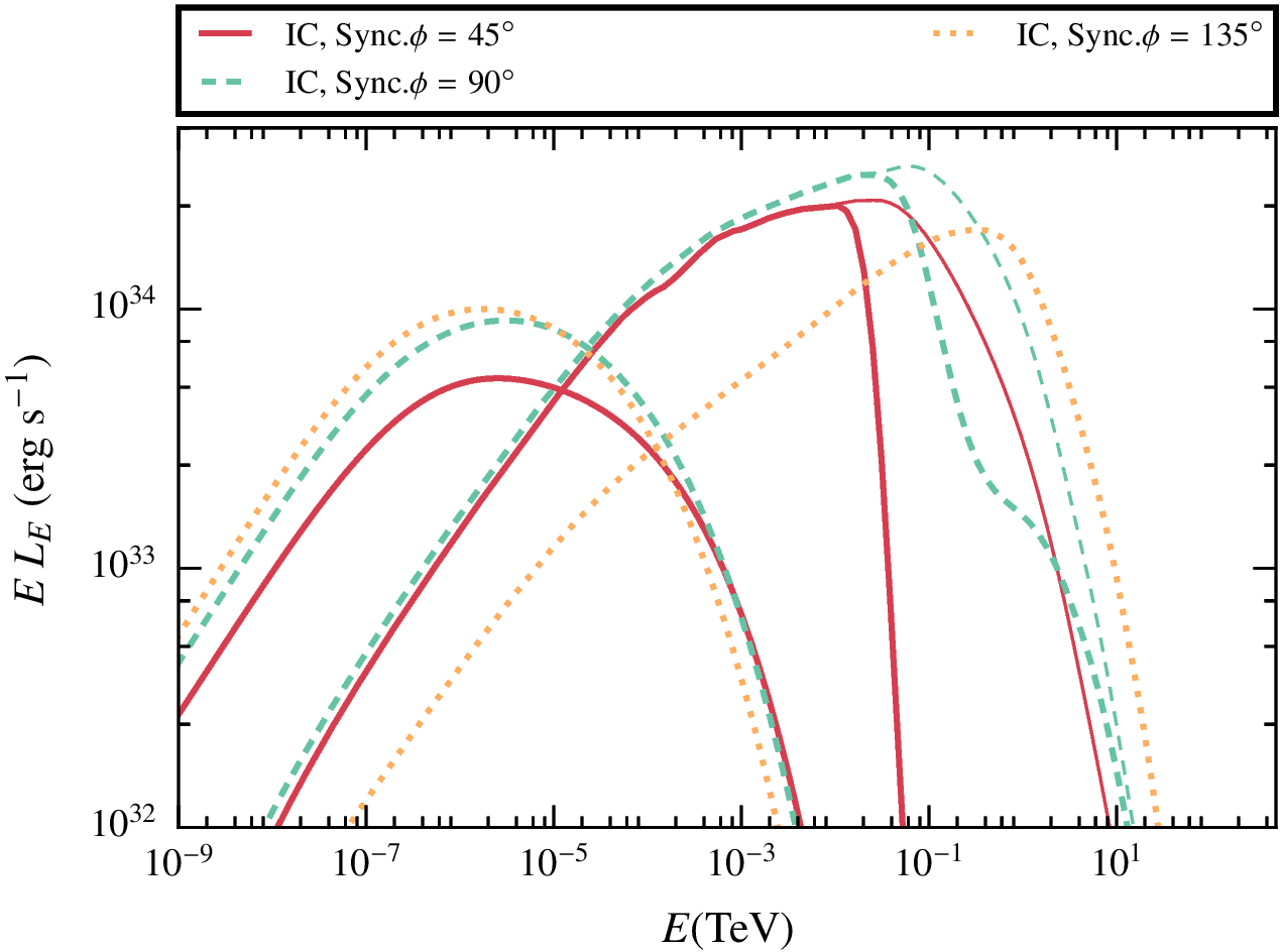
Going into details. observer angle.
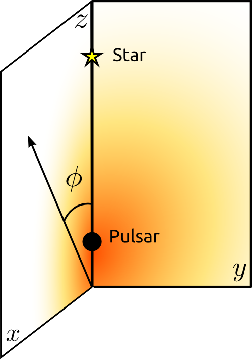
The observer is placed in the z-r plane, forming an angle phi with the z axis.
To avoid eclipses, we do not simulate the extreme angle 0º. Instead, three intermediate angles are studied:
45º, 90º and 135º.
40/59
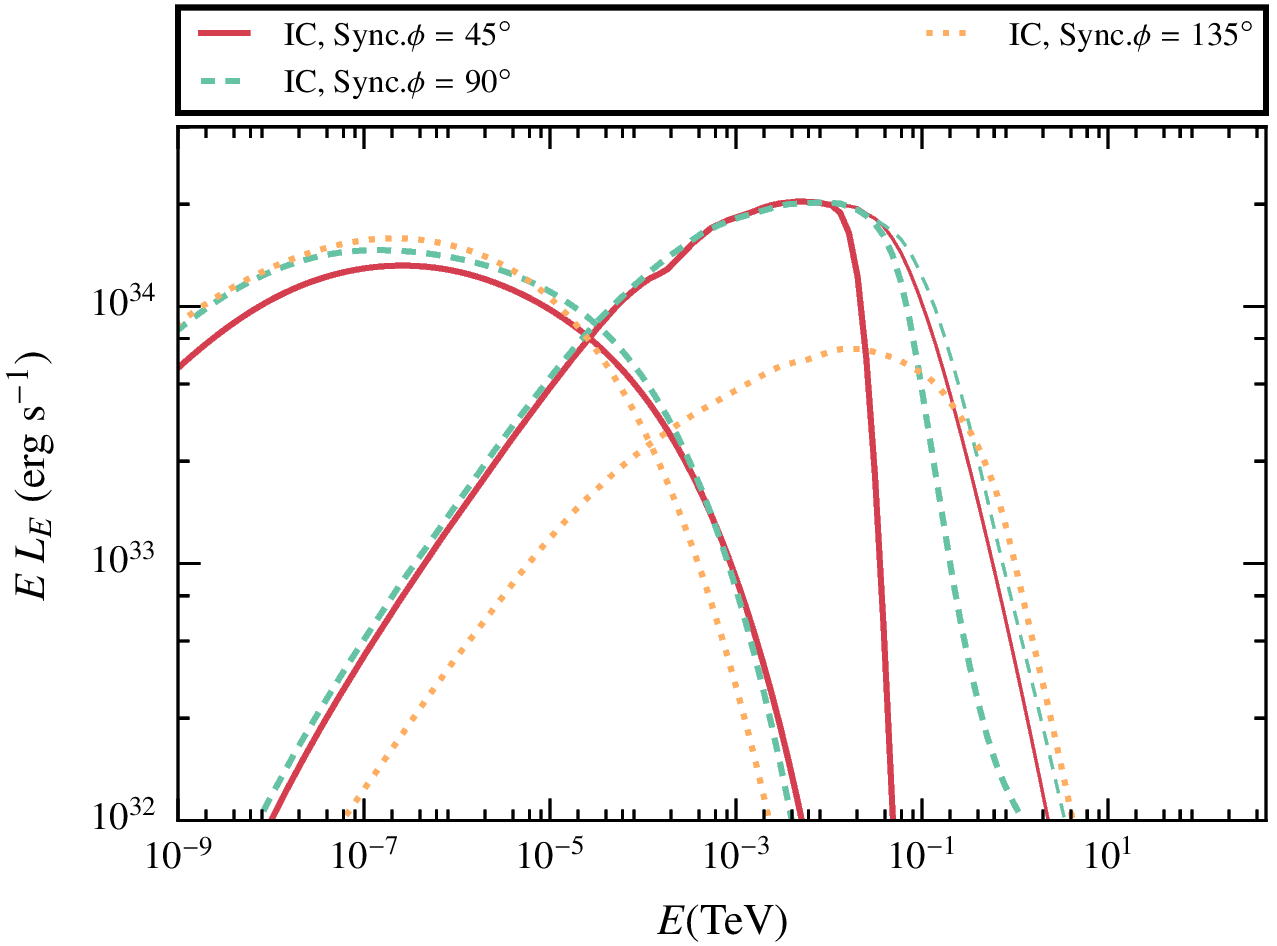
Low B
High B
\chi_B = 10^{-3}
\chi_B = 0.1
Results. two magnetic fields, large clump.
41/59
Results. Extended vs point-like emitter.
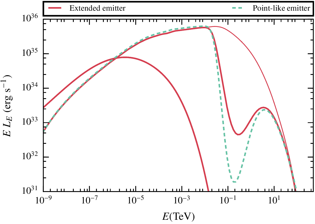
The importance of the hydrodynamic study of the problem is clear when we compare the results obtained assuming a point-like emitter.
A proper characterisation of the emitter is key for the understanding of the SED.
42/59
pulsar wind + clump. conclusions.
V. M. de la Cita, V. Bosch-Ramon, X. Paredes-Fortuny, D. Khangulyan and M. Perucho A&A 598, A13 (2017)
- The Doppler boosting effect is very important in the understanding of these systems.
- Strong instabilities take place easily, and together with the Doppler effect a short-time variable output is expected.
- The main effect of the clump is to move the shocked region closer to the pulsar, which affects the radiation normalisation and SED shape.
43/59
Outline
-
star-jet interactions in active galactic nuclei
-
pulsar wind interacting with a clumpy stellar wind
-
clumpy wind-jet interacions in high-mass microquasars
-
Concluding remarks
-
sources with relativistic outflows moving in rich environments
-
Methods: coupling hydrodynamics and NT calculation
-
Three relevant cases of study:
44/59
high-mass Microquasars (HMMQ)
- Microquasar jets: the donor star transfers matter to the compact object, forming an accretion disk around it and two relativistic jets.
- High-mass microquasar: the winds of the massive donor star (O, B type) are expected to be strongly inhomogeneous, presenting overdensities (clumps) that may interact with the jet.
Owocki & Cohen '06, Moffat '08
45/59
gamma ray emission. cygnus x-1 and cygnus x-3
Cygnus X-1
Cygnus X-3
AGILE Collaboration
Both detected in GeV by Fermi satellite, when the jet is present
46/59
physical scenario
Credit: F. Mirabel
- Proposed by Owocki et al. 2009, first analytical estimates by Araudo et al. 2009 and detailed three-dimensional simulations by Perucho & Bosch-Ramon 2012
- Here we couple for the first time relativistic hydrodynamical (RHD) simulations with non-thermal radiative calculations.
- Along with a semi-analytical description of the frequency and characteristics of this jet-clumps interactions.
47/59
first considerations. jet penetrability.
R_{cl} > 3\times10^{10} \left(\frac{\theta_{j}}{0.1}\right) \left(\frac{10}{\chi}\right) \left(\frac{R_{orb}}{3\times10^{12}\mathrm{cm}}\right) \mathrm{cm}
The minimum radius for a clump to enter the jet is:
The maximum jet luminosity not to destroy the jet before it enters:
L_j < 1.4\times 10^{37} \, \big(\frac{\Gamma_j-1}{\Gamma_j}\big) \big(\frac{\chi}{10}\big) \big(\frac{\dot{M}_w}{3\times 10^{-6} M_\odot \text{yr}^{-1}}\big)
\big(\frac{\theta_j}{0.1}\big)^2 \big(\frac{v_w}{10^8 \text{cm s}^{-1}}\big)\big(\frac{v_j}{c}\big)^{-1} \text{erg} \, \text{s}^{-1}
jet half opening angle
contrast density
orbital radius
R_{cl}

L_{j}
stellar wind speed
jet Lorentz factor
stellar mass-loss rate
2\theta_{j}
\frown
\rho_{cl}/\rho_w
48/59
Jet
direction
L_\text{jet} \sim 10^{37}\text{ erg s}^{-1}
\Gamma = 2
\vec{v}_\text{stellar wind} = 2000 \text{ km s}^{-1}
\dot{M}_\star = 3 \times 10^{-6} M_\odot \text{yr}^{-1}
O-type Star
x_\star = (-3,-3)\times 10^{12} \mathrm{cm}
49/59

~8.5 min
~1 min
~12 min
~10 min
~14 min
First stage
Second stage
50/59
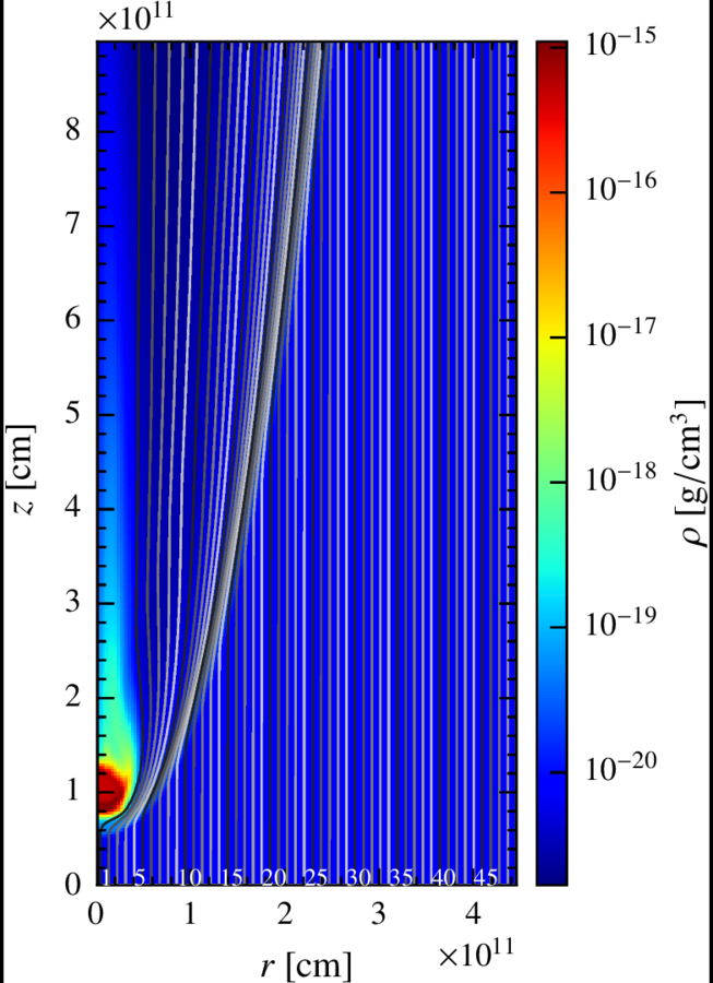
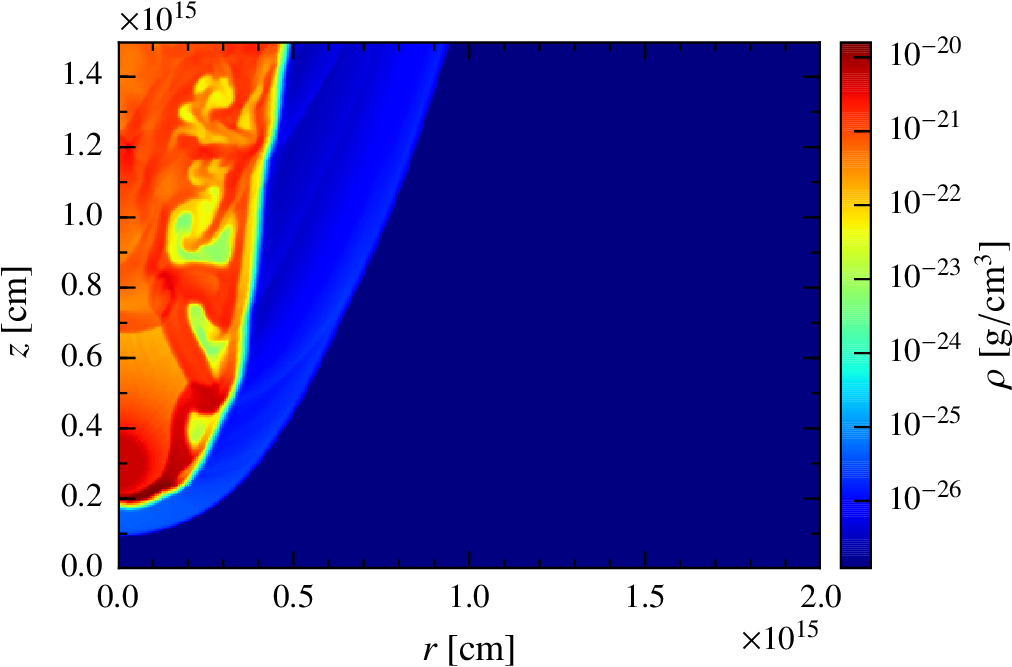
Going into details. hydrodynamic setup.
The fluid is divided in 50 lines with 200 cells each, describing an axisymmetric 2D space of:
r\in[0,4.5]\times10^{11}\text{ cm}
y\in[0,9]\times10^{11}\text{ cm}
The clump radius, height and density contrast are:
r_{cl}=3\times10^{10}\text{ cm}
z_{cl}=3\times10^{12}\text{ cm}
\chi=10
51/59
Going into details. Physical assumptions.
Magnetic field:
\dfrac{B_0^{\prime 2}}{4\pi} = \chi_B (\rho_0hcv)
\chi_B = 10^{-3}, 1
Definition of the magnetic field at the beginning of the line:
(Low, high magnetic field)
Fraction of matter energy flux that goes to magnetic energy
Photon field:
T_{\star} = 4\times 10^4 \text{ K}
L_{\star} = 1\times 10^{39} \text{erg s}^{-1}
52/59
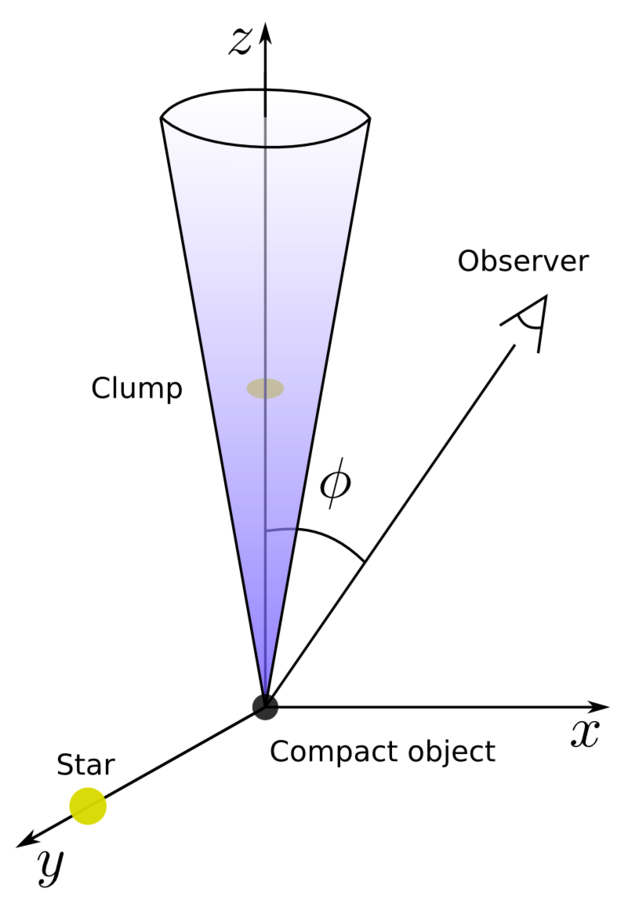
Going into details. Observer angle.
To get a feeling of the importance of the observer angle, we have chosen the following angles:
- 0º - with the jet pointing at the observer
- 30º - representative of Cygnus X-1
- 90º - the observer is placed in the x axis
The observer will be placed in the x axis forming an angle phi with the vertical axis.
\phi = 0^\circ, 30^\circ, 90^\circ
53/59
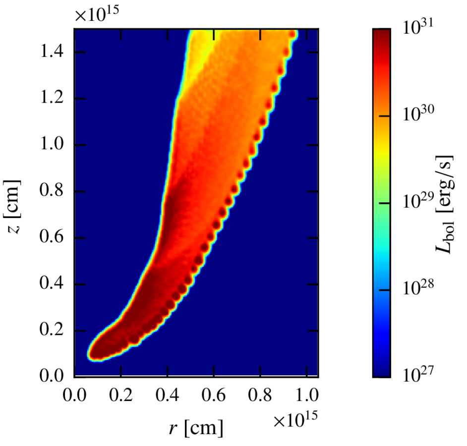
Results. First case, smaller shocked region
In the case of a low magnetic field, the IC radiation dominates the spectrum.
The difference between the three angles come from the doppler boosting, more important for smaller angles given that most of the cells have a strong z- component of the velocity
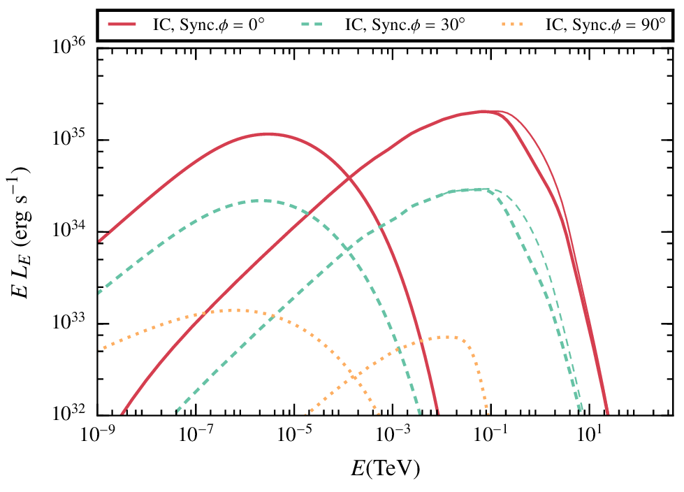
Low B
High B
\chi_B = 10^{-3}
\chi_B = 1
10^{35} \text{ erg s}^{-1}
54/59
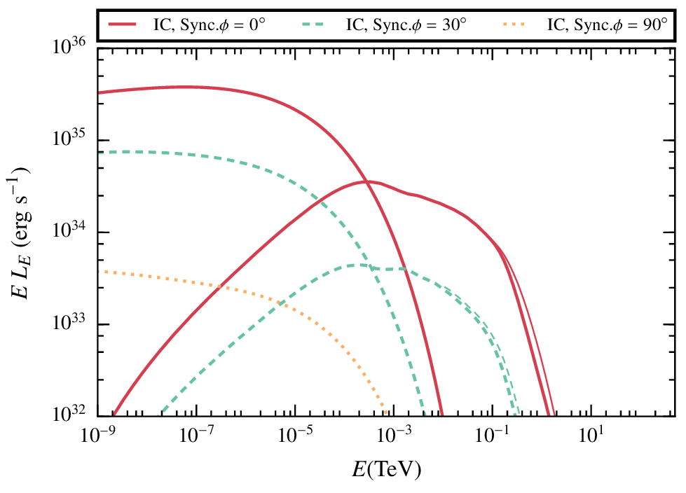
Low B
High B
\chi_B = 10^{-3}, \phi = 30^\circ
\chi_B = 1, \phi = 30^\circ
Results. comparison between the two cases.
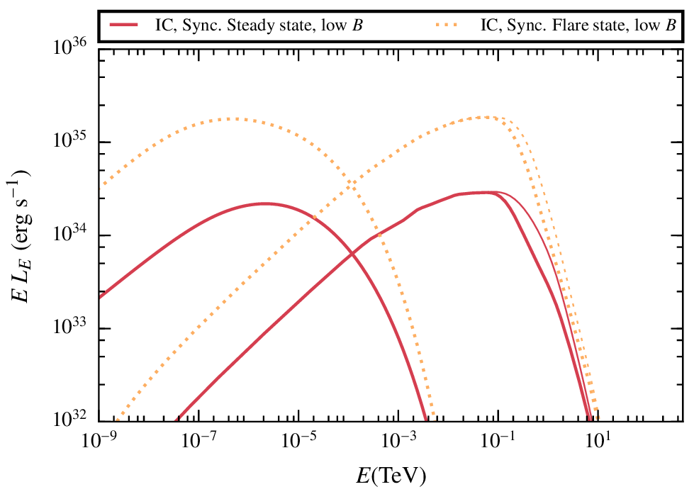
In general the non-thermal radiation will be increased for larger shocks, produced while the clumps is being disrupted.
55/59
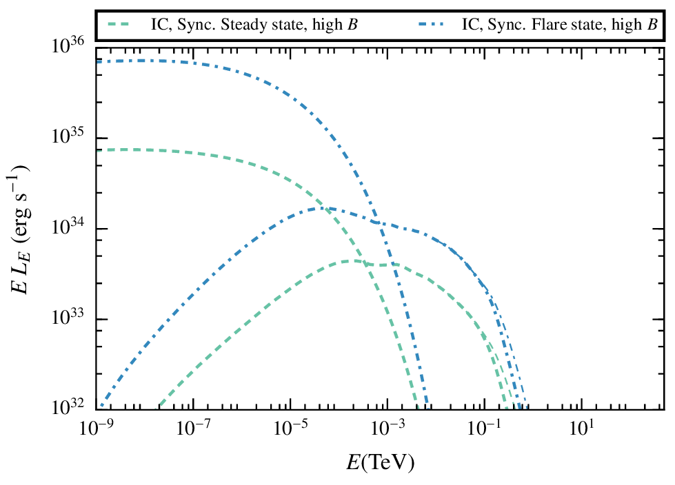
Results. Duty cycle and standing luminosity.
L_\text{GeV}\approx 10^{35} \text{ erg s}^{-1}
Knowing the lifetime of a clump inside the jet and the frequency they enter with (for a given clump size) we can compute the duty cycle (DC): the fraction of the time that a certain type of clumps are interacting with the jet.
For a wide variety of parameters we obtain a duty cycle of 1, meaning there is about one clump interacting with the jet at every time .
\chi = 0.1
DC \sim 1
56/59
Results. Cygnus x-1.
V. M. de la Cita S. del Palacio, V. Bosch-Ramon, X. Paredes-Fortuny, G. E. Romero and D. Khangulyan 2017, accepted for publication in A&A
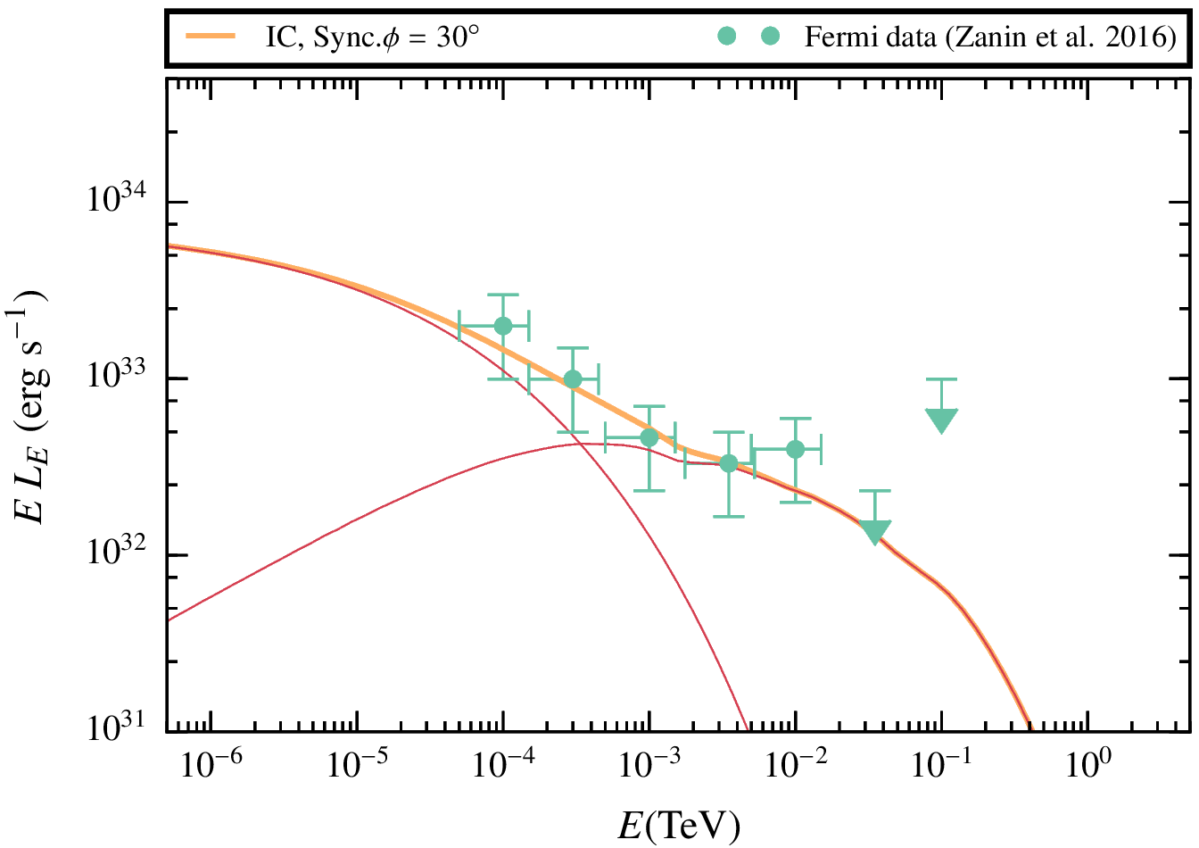
We were able to reproduce the results for Cyg X-1 with a strong magnetic field
and a relatively conservative NT efficiency
\chi_B = 0.5
\chi = 0.01
57/59
Outline
-
star-jet interactions in active galactic nuclei
-
pulsar wind interacting with a clumpy stellar wind
-
clumpy wind-jet interacions in high-mass microquasars
-
Concluding remarks
-
sources with relativistic outflows moving in rich environments
-
Methods: coupling hydrodynamics and NT calculation
-
Three relevant cases of study:
58/59
Concluding remarks
- The complexity of the systems under study demands a proper characterisation of the hydrodynamical properties of the emitter.
- A better understanding of these systems would be possible with the upcoming observational tools (CTA, Athena)
- The next step in our work would imply magneto-hydrodynamic simulations and a proper 3D study of the problem, as well as bigger computational grids.
Thank You.
59/59
Thesis defence
By otnoesmusica
Thesis defence
Coupling fluid-dynamics and non-thermal processes to study sources of high-energy emission


