Contribution due to clumpy winds to the gamma-ray emission in microquasar jets
s. del palacio, v. bosch-ramon, X. paredes-fortuny, g. e. romero and D. khangulyan
Bilbo, 22th July 2016
V. M. DE LA CITA

high-mass Microquasars (HMMQ)
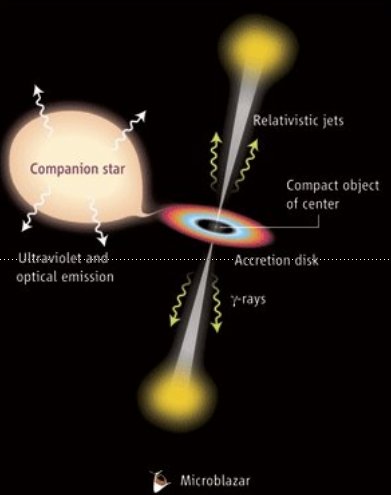
- Microquasar jets: the donor star transfers matter to the compact object, forming an accretion disk around it and two relativistic jets.
- High-mass microquasar: the winds of the massive donor star (O, B type) are expected to be strongly inhomogeneous, presenting overdensities (clumps) that may interact with the jet.
Owocki & Cohen '06, Moffat '08
gamma ray emission. cygnus x-1 and cygnus x-3
Cygnus X-1
Cygnus X-3
AGILE Collaboration
Both detected in GeV by Fermi satellite, when the jet is present
physical scenario
Credit: F. Mirabel
- Proposed by Owocki et al. 09, first analytical estimates by Araudo et al. '09 and detailed three-dimensional simulations by Perucho et al. '12
- Here we couple for the first time relativistic hydrodynamical (RHD) simulations with non-thermal radiative calculations.
- Along with a semi-analytical description of the frequency and characteristics of this jet-clumps interactions.
first considerations. jet penetrability.
R_{cl} > 3\times10^{10} \left(\frac{\theta_{j}}{0.1}\right) \left(\frac{10}{\chi}\right) \left(\frac{R_{orb}}{3\times10^{12}\mathrm{cm}}\right) \mathrm{cm}
The minimum radius for a clump to enter the jet is:
The maximum jet luminosity not to destroy the jet before it enters:
L_j < 1.4\times 10^{37} \, \big(\frac{\Gamma_j-1}{\Gamma_j}\big) \big(\frac{\chi}{10}\big) \big(\frac{\dot{M}_w}{3\times 10^{-6} M_\odot \text{yr}^{-1}}\big)
\big(\frac{\theta_j}{0.1}\big)^2 \big(\frac{v_w}{10^8 \text{cm s}^{-1}}\big)\big(\frac{v_j}{c}\big)^{-1} \text{erg} \, \text{s}^{-1}
jet opening angle
contrast density
orbital radius
R_{cl}

L_{j}
stellar wind speed
jet Lorentz factor
stellar mass-loss rate
\theta_{j}
\frown
Jet
direction
L_\text{jet} \sim 10^{37}\text{ erg s}^{-1}
\Gamma = 2
\vec{v}_\text{stellar wind} = 2000 \text{ km s}^{-1}
\dot{M}_\star = 3 \times 10^{-6} M_\odot \text{yr}^{-1}
O-type Star
x_\star = (-3,-3)\times 10^{12} \mathrm{cm}

~8.5 min
~1 min
~12 min
~10 min
~14 min
First stage
Second stage
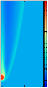
Going into details. hydrodynamic setup.
The fluid is divided in 50 lines with 200 cells each, describing an axisymmetric 2D space of:
r\in[0,4.5]\times10^{11}\text{ cm}
y\in[0,9]\times10^{11}\text{ cm}
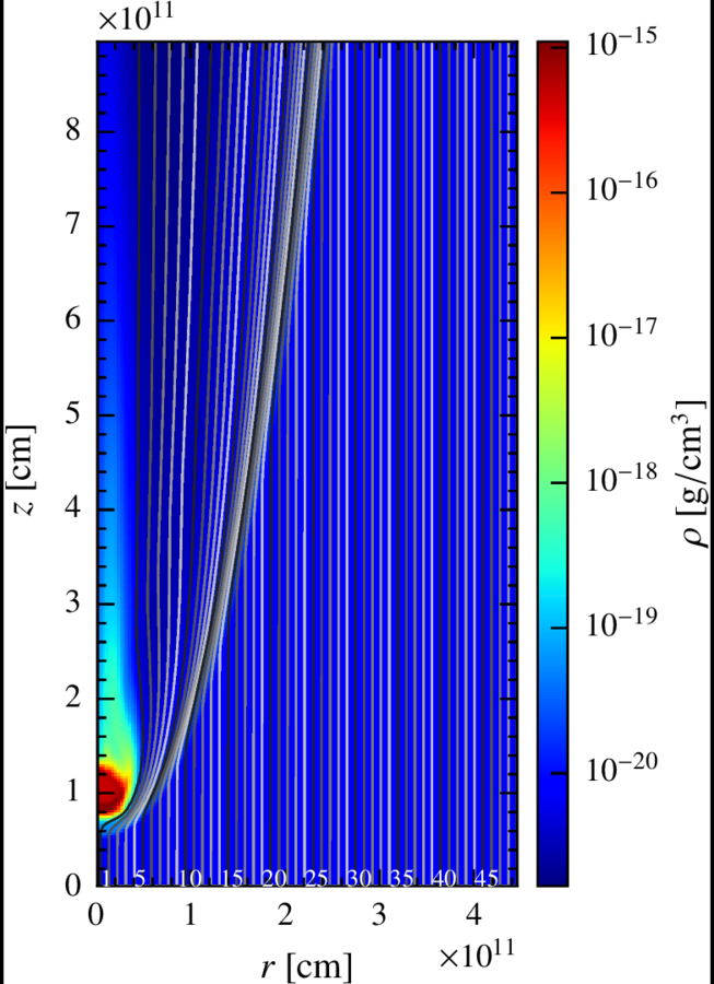
The clump radius, height and density contrast are:
r_{cl}=3\times10^{10}\text{ cm}
z_{cl}=3\times10^{12}\text{ cm}
\chi=10
Half the solar radius
A fifth of an Astronomical Unit
Although the RHD simulation is 2D, we take this information and scramble the different lines around the y axis, giving each cell a random azimuthal angle phi, so the result is more similar to the 3D real scenario.
Going into details. 3d emitter.

de la Cita et al. 2016
Going into details. Physical assumptions.
Magnetic field perpendicular to the fluid line
\dfrac{B_0^{\prime 2}}{4\pi} = \chi_B (\rho_0h_0c^2)
B_k^\prime = B_0^\prime \Big( \dfrac{\rho_k v_0\Gamma_0}{\rho_0 v_k \Gamma_k}\Big)^{1/2}
\chi_B = 10^{-4}, 1
Definition of the magnetic field at the beginning of the line:
Evolution of the B field in the different cells k:
(Low, high magnetic field)
Fraction of matter energy flux that goes to magnetic energy
Photon field:
T_{\star} = 4\times 10^4 \text{ K}
L_{\star} = 1\times 10^{39} \text{erg s}^{-1}
injection of non-thermal particles
A fraction of the generated internal energy per second in the cell k enters in the form of non-thermal particles.
\chi = 0.1
Biggest uncertainty
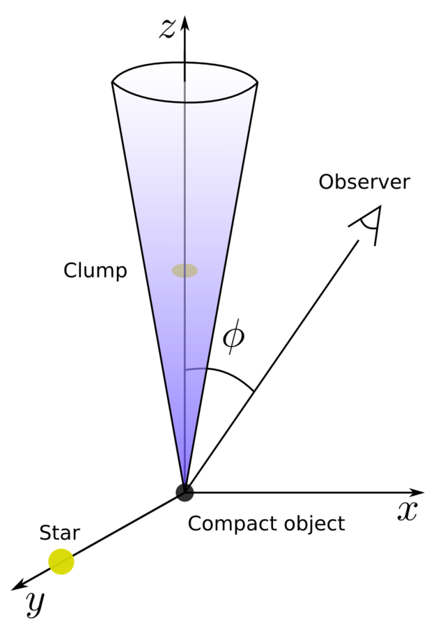
Going into details. Observer angle.
To get a feeling of the importance of the observer angle, we have chosen the following angles:
- 0º - with the jet pointing at the observer
- 30º - representative of Cygnus X-1
- 90º - the observer is placed in the x axis
The observer will be placed in the x axis forming an angle phi with the vertical axis.
\phi = 0^\circ, 30^\circ, 90^\circ
Going into details. some notes on the code.
-
We let the particles evolve until they reach a steady state so we can consider the medium stationary, in other words, every loss time (e.g. synchrotron) or cell-crossing time is much shorter than the dynamical time on large scales. Described in de la Cita et al. '16.
-
All the computation is done in the (relativistic) frame of the fluid, so every relevant quantity has to be transformed, including the angles between fluid, gamma photons and target photons velocities.
-
Once we have the electron distribution, we compute the inverse Compton (IC) and synchrotron radiation, taking into account the Doppler boosting.
\delta = 1/\Gamma(1-\beta\cos{\theta_\text{obs}})
\epsilon L(\epsilon)= \delta^4\epsilon'L'(\epsilon')
where
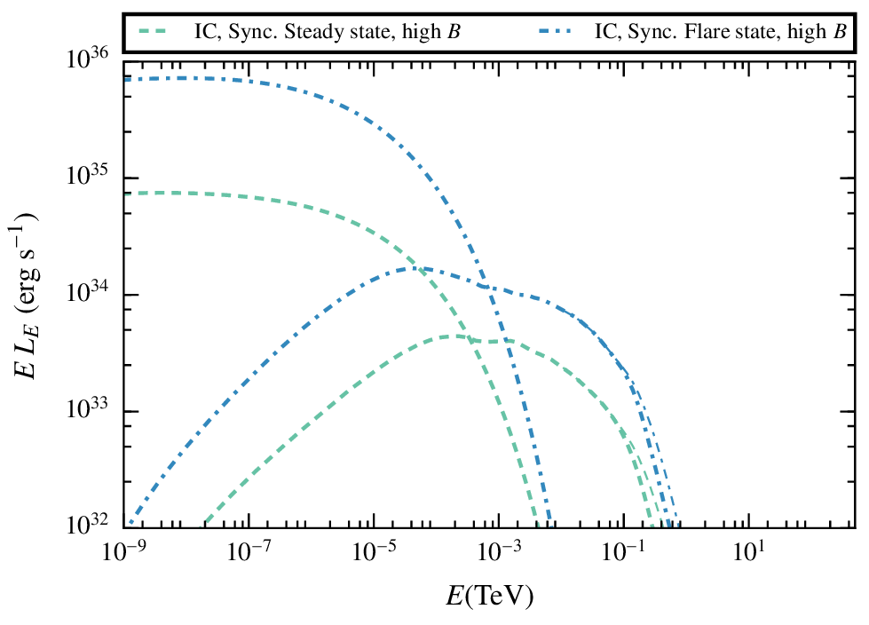
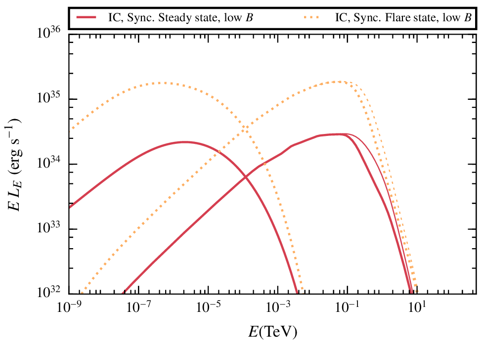
Results. First case, smaller shocked region
In the case of a low magnetic field, the IC radiation dominates the spectrum.
The difference between the three angles come from the doppler boosting, more important for smaller angles given that most of the cells have a strong z- component of the velocity
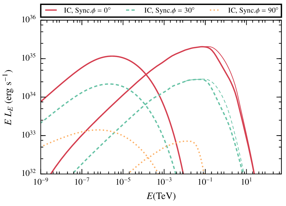
Low B
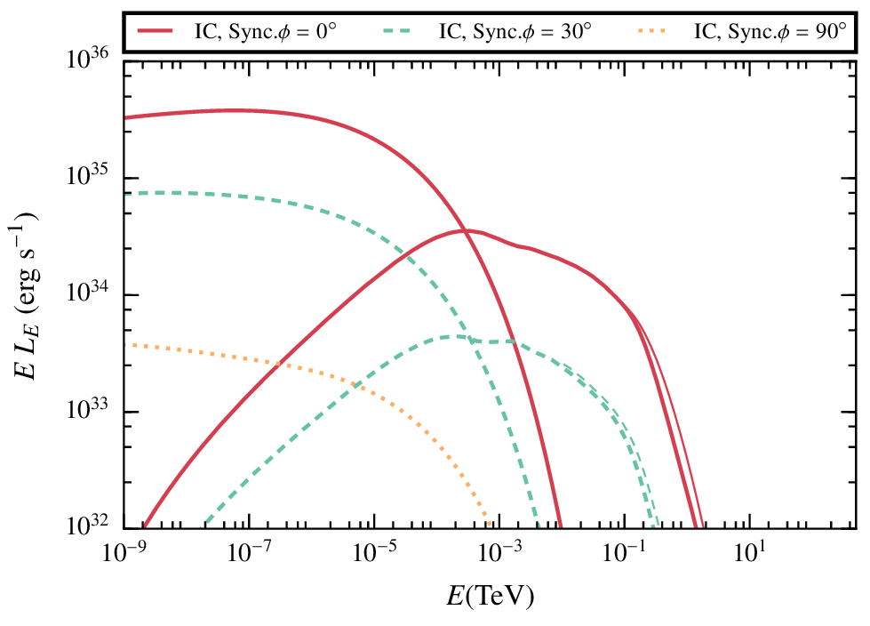
High B
\chi_B = 10^{-4}
\chi_B = 1
10^{35} \text{ erg s}^{-1}
Low B
High B
\chi_B = 10^{-4}, \phi = 30^\circ
\chi_B = 1, \phi = 30^\circ
Results. comparison between the two cases.
In general the non-thermal radiation will be increased for larger shocks, produced while the clumps is being disrupted.
Results. Duty cycle and standing luminosity.
L_\text{GeV}\approx 10^{35} \text{ erg s}^{-1}
Knowing the lifetime of a clump inside the jet and the frequency they enter with (for a given clump size) we can compute the duty cycle (DC): the fraction of the time that a certain type of clumps are interacting with the jet.
For a wide variety of parameters we obtain a duty cycle of 1, meaning there is about one clump interacting with the jet at every time .
Cygnus X-1:
Cygnus X-3:
\chi \sim 0.01
\chi \sim 0.1
DC \sim 1
Conclusions.
-
The effective radius of the emitter is much bigger than the clump radius. Emission levels strongly depend on the viewer angle due to Doppler boosting.
-
Depending on the duty cycle and the mass distribution of clumps, their radiation can contribute to either the standing high-energy emission.
-
...and also be responsible of short GeV flares, like those observed by AGILE in Cygnus X-1 (Sabatini et al. '10).
eskerrik asko.
backup slide. Physical assumptions.
We follow a prescription for particle acceleration in strong shocks. The acceleration timescale goes like ~1/v² as proposed in previous works (e.g. Drury 1983)
We inject non-thermal particles when a shock takes place:
Internal energy goes up
and
fluid velocity goes down
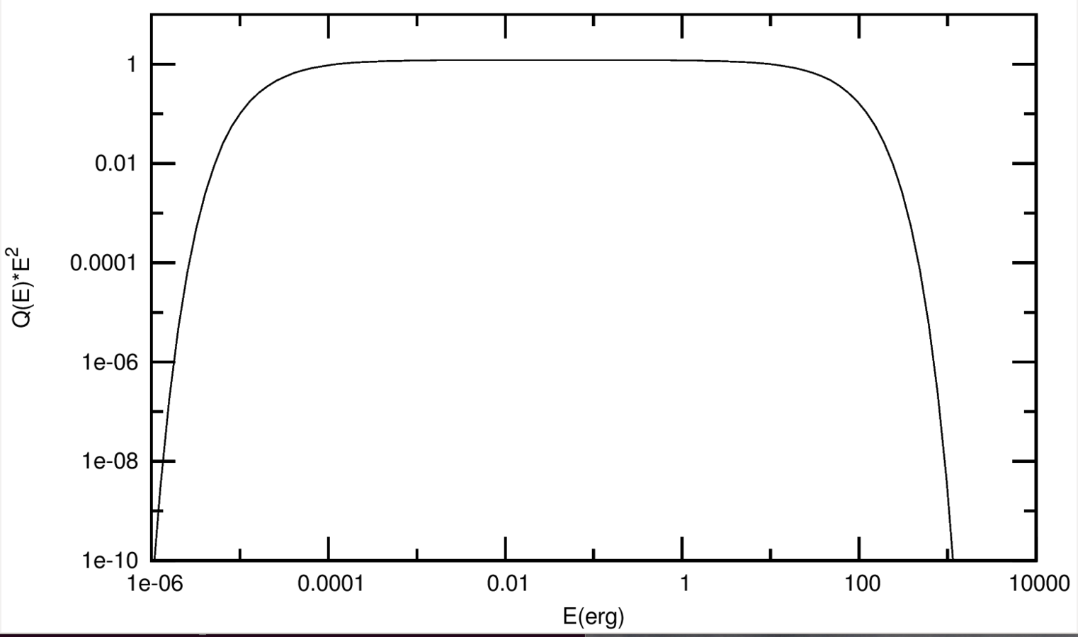
Where and how do we inject non-thermal particles
Q(E) \propto E^{-2} \times (e^{-E_{min}/E})^5 \times e^{-E/E_{max}}
t'_\text{acc}=\eta E'qB'c, \text{with}
\eta = 2\pi (c/v)^2
Backup slide. Fixing the line ending.
Given that the two winds can mix through the fluid lines, we have had to cut the lines at a certain point. To do so, we can impose that the amount of material that crosses the section do not get larger than a certain threshold:
\text{if: } S\rho v\Gamma > 2\times S_0\rho_0v_0\,\rightarrow\, \text{end of the line}
Backup slide. Injected Luminosity.
The injected non-thermal particles have a lumisosity given by a fraction of the generated internal energy per second in the cell.
L_{inj} = \chi_{NT} \times \dot{U}'_k =
With the pre-factor varying between 0 and 1 and the +/- subindexes refering to the right/left boundaries, respectively.
= \chi_{NT} v_k\Gamma_k^2\times \left(S_+\Gamma_+^2h_+\rho_+c^2\left(1 +\dfrac{v_+^2}{c^2}\right) - S_-\Gamma_-^2h_-\rho_-c^2\left(1 +\dfrac{v_-^2}{c^2}\right)\right)
Bilbao 2016
By otnoesmusica
Bilbao 2016
Contribution due to clumpy winds to the gamma-ray emission in microquasar jets


