Phase-type models in life insurance
and empirical dynamic modelling
Patrick J. Laub
University of Melbourne
Outline
- Mention some past work
- Phase-type distributions in life insurance
- Describe some current work (EDM)


Phil Pollett
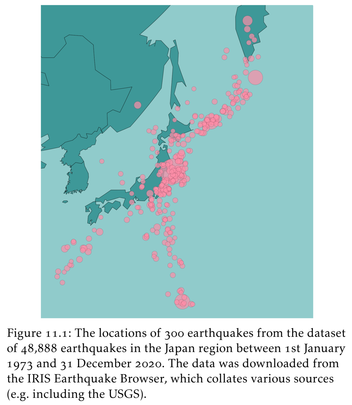
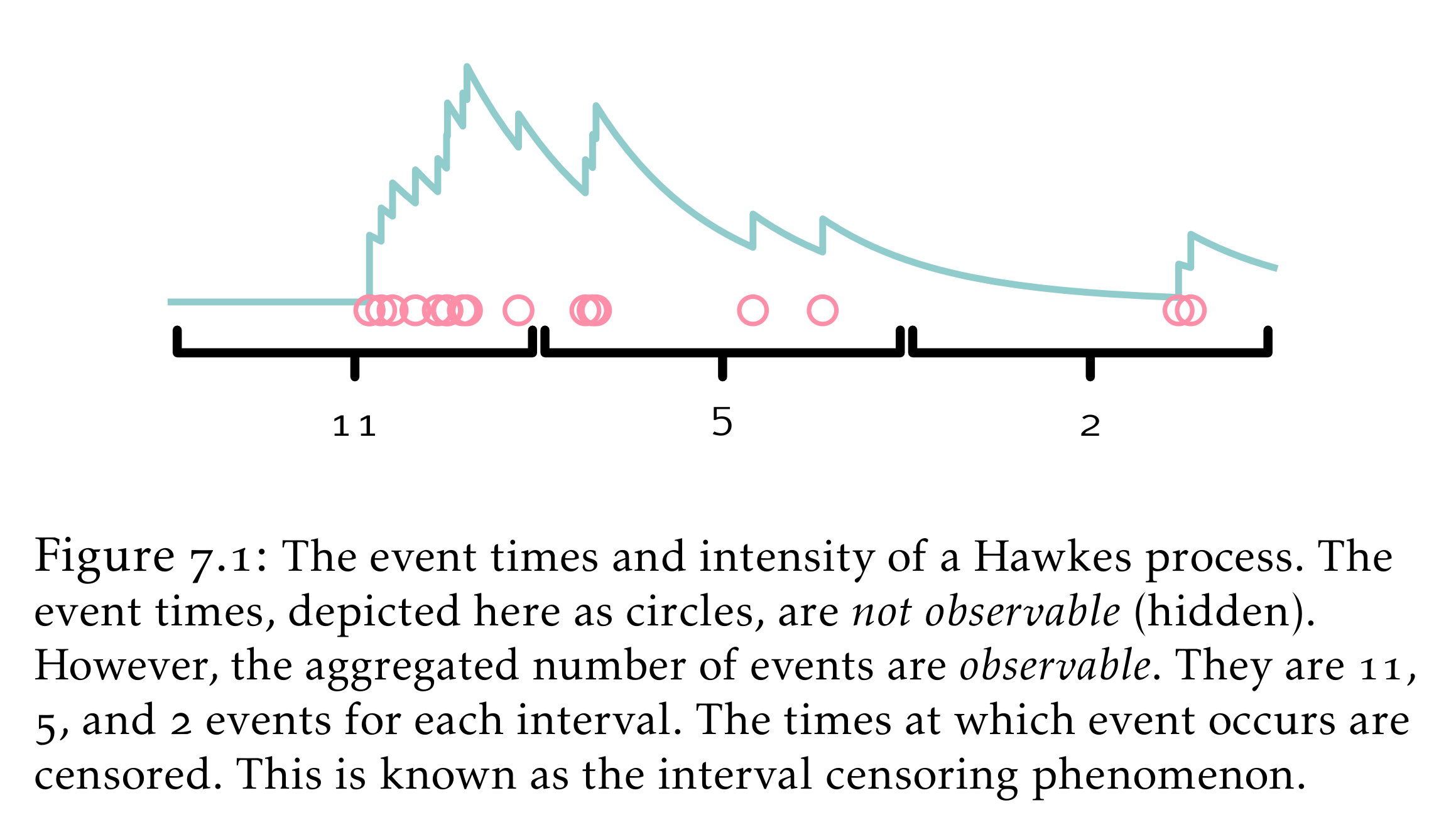
Hawkes processes
Sums of random variables
S = X_1 + X_2
f_S(s) = \int_{-\infty}^{\infty} f_{X}(x_1) f_{X}(s - x_1) \, \mathrm{d} x_1
X_1,X_2 \overset{\text{i.i.d.}}{\sim} f_X(\cdot)
Cramér-Lundberg model
Useful for:
- Ruin probability (finite time)
- Ruin probability (infinite time)
- Stop-loss premiums
- Option pricing
Sum of lognormals distributions
S = X_1 + X_2 + \ldots + X_d
X \sim \mathsf{Lognormal}(\mu, \Sigma)
where
S \sim \mathsf{SumLognormal}(\mu, \Sigma)
Advances in Applied Probability, 48(A)
"I used to be a chick[en] but am less so as I get older. After all, I have to die from something."
Savage condition
\text{minimise } x^\top \Sigma^{-1} x \text{ under the linear constraint } x \ge 1
\text{Savage condition} \equiv \Sigma^{-1} 1 > 0
Hashorva, E. (2005), 'Asymptotics and bounds for multivariate Gaussian tails', Journal of Theoretical Probability
Pierre-Olivier Goffard, Patrick J. Laub (2020), Orthogonal polynomial expansions to evaluate stop-loss premiums, Journal of Computational and Applied Mathematics
S = X_1 + \ldots + X_N
Orthogonal polynomials
Approximate S using orthogonal polynomial expansion
= \sum_{i=0}^{\infty} p_i \gamma(r+i,m,x)
\gamma(\alpha,\beta,x) = \text{PDF}(\mathsf{Gamma}(\alpha,\beta), x)
f_{X}(x)=\sum_{k=0}^{\infty} q_k Q_{k}(x) f_\nu(x)
where

Pierre-O Goffard
Stop-loss premiums
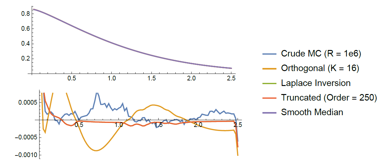
N\sim\mathsf{Poisson}(\lambda=2) \text{ and } U\sim\mathsf{Gamma}(r=3/2,m=1/3)
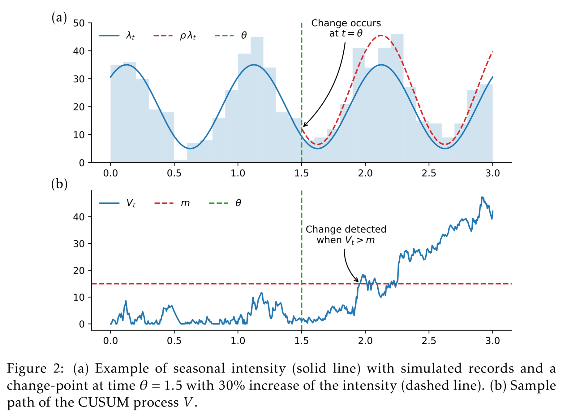

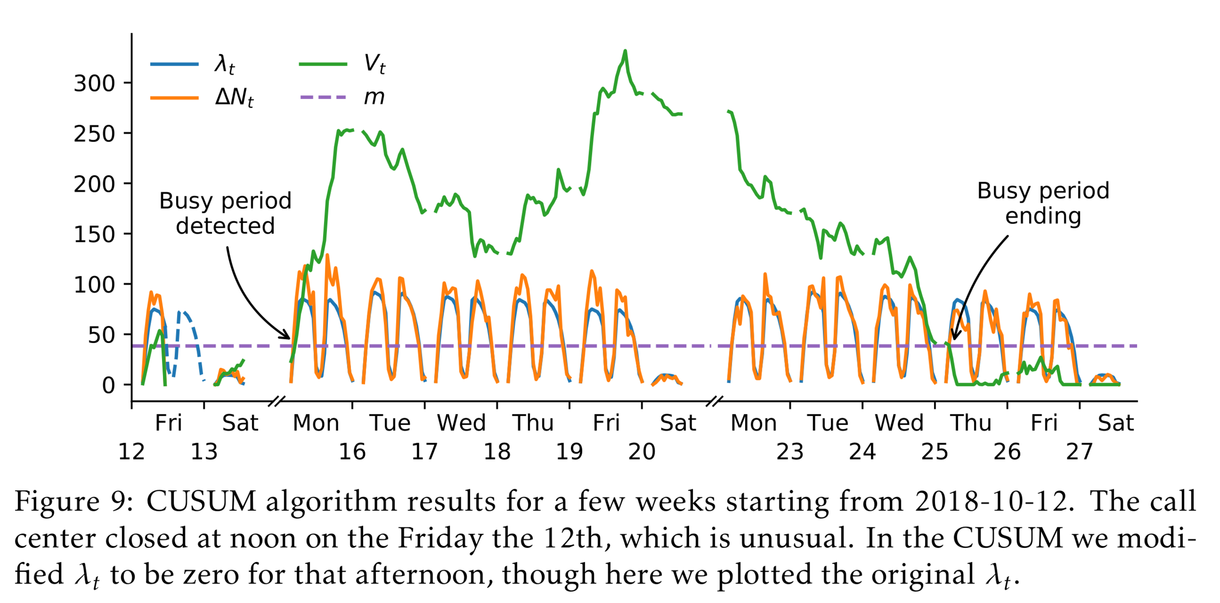
Change-point detection
Approximate Bayesian Computation
Time-varying example
- Claims form a Poisson process point with arrival rate \( \lambda(t) = a+b[1+\sin(2\pi c t)] \).
- The observations are \( X_s = \sum_{i = N_{s-1}}^{N_{s}}U_i \).
- Frequencies are \(\mathsf{CPoisson}(a=1,b=5,c=\frac{1}{50})\) and sizes are \(U_i \sim \mathsf{Lognormal}(\mu=0, \sigma=0.5)\).


a
b
c
\mu
\sigma
\mathcal{D}(\cdot, \cdot) \text{ is Wasserstein distance}
\mathcal{D}(\cdot, \cdot) \text{ is } L^1 \text{ of sorted data}
- Claims form a Poisson process point with arrival rate \( \lambda(t) = a+b[1+\sin(2\pi c t)] \).
- The observations are \( X_s = \sum_{i = N_{s-1}}^{N_{s}}U_i \).
- Frequencies are \(\mathsf{CPoisson}(a=1,b=5,c=\frac{1}{50})\) and sizes are \(U_i \sim \mathsf{Lognormal}(\mu=0, \sigma=0.5)\).
- ABC posteriors based on 50 \(X\)'s and on 250 \(X\)'s with uniform priors.
Wasserstein distance?
\mathcal{W}_p(\bm{x},\tilde{\bm{x}}) = \Bigl( \underset{\sigma\in\mathcal{S}_t}{\inf}\frac 1n\sum_{s=1}^{t}\, \rho(x_{s},\tilde{x}_{\sigma(s)})^p \Bigr)^{1/p},
where \(\mathcal{S}_t\) denotes the set of all the permutations of \(\{1,\ldots, t\}\).
\mathcal{W}_1(\bm{x},\tilde{\bm{x}}) = \sum_{i=1}^n | x_{(i)} - \tilde{x}_{(i)} |
One-dimensional data:
Sorting is only \( \mathcal{O}(n \log n) \)

Compare \(\boldsymbol{x}_{\text{obs}} \sim f(\cdot, \boldsymbol{\theta}) \) to \(\boldsymbol{y} \sim f(\cdot, \boldsymbol{\theta}) \)

Normal Wasserstein distance ignores time

\( L^1 \) distance strictly enforces time
a
b
c
\mu
\sigma
\mathcal{D}(\cdot, \cdot) \text{ is curve-matching distance}
- Claims form a Poisson process point with arrival rate \( \lambda(t) = a+b[1+\sin(2\pi c t)] \).
- The observations are \( X_s = \sum_{i = N_{s-1}}^{N_{s}}U_i \).
- Frequencies are \(\mathsf{CPoisson}(a=1,b=5,c=\frac{1}{50})\) and sizes are \(U_i \sim \mathsf{Lognormal}(\mu=0, \sigma=0.5)\).
- ABC posteriors based on 50 \(X\)'s and on 250 \(X\)'s with uniform priors.
\rho_\gamma(x_i,\tilde{x}_j) = \sqrt{(x_i - \tilde{x}_j)^2 + \gamma^2(i-j)^2}

We can scale time to balance the two axes
Jevgenijs Ivanovs

\tau
S_t
t
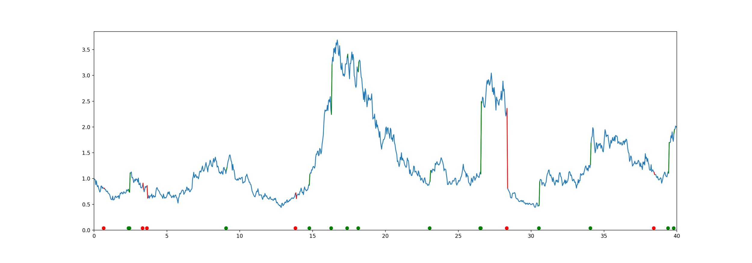
Guaranteed Minimum Death Benefit
S_\tau
\text{Payoff} = \max( S_{\tau}, K )
Equity-linked life insurance
\tau
t
High Water Death Benefit
\text{Payoff} = \overline{S}_{\tau}
Equity-linked life insurance
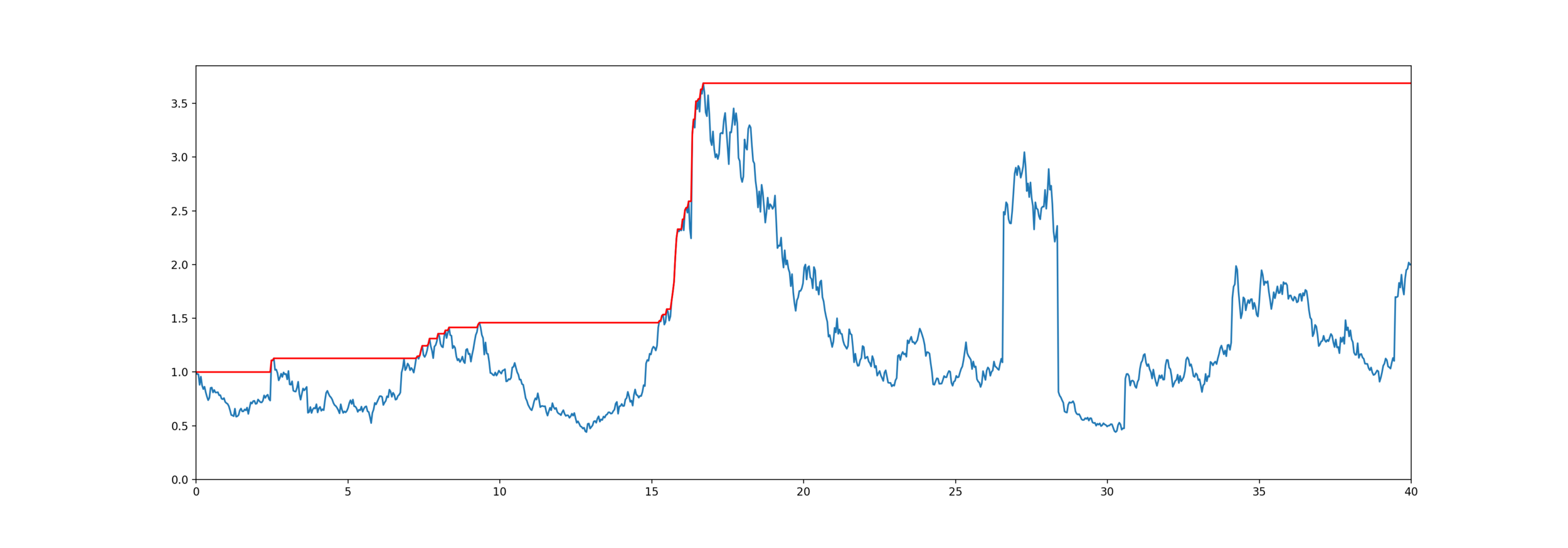
\overline{S}_\tau
\overline{S}_t = \max_{s \le t} S_s
Model for mortality and equity
The customer lives for years,
\tau
\tau \sim \text{PhaseType}(\boldsymbol{\alpha}, \boldsymbol{T})
X_t \sim \text{Jump Diffusion}
S_t = S_0 \mathrm{e}^{X_t}
The stock price is an exponential jump diffusion,
\text{Brownian Motion}(\mu, \sigma^2) + \text{Compound Poisson}(\lambda_1) + \text{Compound Poisson}(\lambda_2)
\text{Price} = \mathbb{E}[ \mathrm{e}^{-\delta \tau} \text{Payoff}( S_\tau, \overline{S}_\tau ) ]
S_t
t
Exponential PH-Jump Diffusion
\text{UpJumpSize}_i \overset{\mathrm{i.i.d.}}{\sim} \text{PhaseType}(\boldsymbol{\alpha}_1, \boldsymbol{T}_1)
\text{DownJumpSize}_i \overset{\mathrm{i.i.d.}}{\sim} \text{PhaseType}(\boldsymbol{\alpha}_2, \boldsymbol{T}_2)
Wiener-Hopf Factorisation
\mathbb{P}(\overline{X}_\tau \in \mathrm{d}x, X_\tau - \overline{X}_\tau \in \mathrm{d}y) = \mathbb{P}(\overline{X}_\tau \in \mathrm{d}x) \mathbb{P}(\underline{X}_\tau \in \mathrm{d}y)
X_t
-
is an exponential random variable
- is a Lévy process
\tau
Doesn't work for deterministic time
IME Papers by Gerber, Hans U., Elias S. W. Shiu, and Hailiang Yang:
- Valuing equity-linked death benefits and other contingent options: A discounted density approach (2012)
- Valuing equity-linked death benefits in jump diffusion models (2013)
- Geometric stopping of a random walk and its application to valuation of equity-linked death benefits (2015)
Problem: to model mortality via phase-type
Bowers et al (1997), Actuarial Mathematics, 2nd Edition


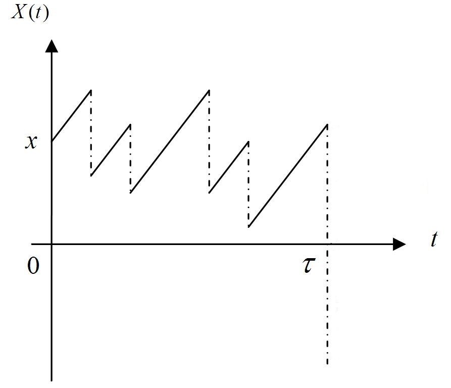
t
X_t
Example Markov process
( X_t )_{t \ge 0}
Sojourn times
Sojourn times are the random lengths of time spent in each state

S_1
S_2
S_3
S_5^{(1)}
S_5^{(2)}
S_1 \sim \mathsf{Exp}(1/\mu_1)
S_2 \sim \mathsf{Exp}(1/\mu_2)
S_5^{(1)}, S_5^{(2)} \overset{\mathrm{i.i.d.}}{\sim} \mathsf{Exp}(1/\mu_5)
S_4
Phase-type definition
Markov process State space
- Initial distribution
- Sub-transition matrix
- Exit rates
\boldsymbol{\alpha}
\boldsymbol{T}
\boldsymbol{t} = -\boldsymbol{T} 1
\boldsymbol{t}
\tau = \inf_t \{ X_t = \dagger \}
( X_t )_{t \ge 0}
\{1, ..., p, \dagger \}
\Leftrightarrow \tau \sim \mathrm{PhaseType}(\boldsymbol{\alpha}, \boldsymbol{T})
\boldsymbol{Q} = \begin{bmatrix}
\boldsymbol{T} & \boldsymbol{t} \\
0 & 0
\end{bmatrix}
\dagger
1
3
2
\boldsymbol{Q} = \begin{bmatrix}
-6 & 4 & 2 & 0 \\
1 & -1 & 0 & 0 \\
0 & 5 & -5.5 & 0.5 \\
0 & 0 & 0 & 0
\end{bmatrix}
\boldsymbol{\alpha} = [ \frac13, \frac13, \frac13, 0 ]^\top
2
4
1
0.5
5
Example
Markov process State space
( X_t )_{t \ge 0}
\{1, 2, 3, \dagger \}
\boldsymbol{T} = \begin{bmatrix}
-6 & 4 & 2 \\
1 & -1 & 0 \\
0 & 5 & -5.5
\end{bmatrix}
\boldsymbol{t} = \begin{bmatrix}
0 \\
0 \\
0.5
\end{bmatrix}
Phase-type generalises...
- Exponential distribution
- Sums of exponentials (Erlang distribution)
- Mixtures of exponentials (hyperexponential distribution)
\boldsymbol{\alpha} = [ 1 ], \boldsymbol{T} = [ -\lambda ], \boldsymbol{t} = [ \lambda ]
\boldsymbol{\alpha} = \begin{bmatrix}
1 \\
0 \\
0
\end{bmatrix} ,
\boldsymbol{T} = \begin{bmatrix}
-\lambda_1 & \lambda_1 & 0 \\
0 & -\lambda_2 & \lambda_2 \\
0 & 0 & -\lambda_3
\end{bmatrix}
, \boldsymbol{t} = \begin{bmatrix}
0 \\
0 \\
\lambda_3
\end{bmatrix}
\boldsymbol{\alpha} = \begin{bmatrix}
\alpha_1 \\
\alpha_2 \\
\alpha_3
\end{bmatrix} ,
\boldsymbol{T} = \begin{bmatrix}
-\lambda_1 & 0 & 0 \\
0 & -\lambda_2 & 0 \\
0 & 0 & -\lambda_3
\end{bmatrix}
, \boldsymbol{t} = \begin{bmatrix}
\lambda_1 \\
\lambda_2 \\
\lambda_3
\end{bmatrix}
Phase-type properties
Matrix exponential
Density and tail
Moments
Laplace transform
f_\tau(s) = \boldsymbol{\alpha}^\top \mathrm{e}^{\boldsymbol{T} s} \boldsymbol{t}
\mathrm{e}^{\boldsymbol{T} s} = \sum_{i=0}^\infty \frac{(\boldsymbol{T} s)^i}{i!}
\tau \sim \mathrm{PhaseType}(\boldsymbol{\alpha}, \boldsymbol{T})
\overline{F}_\tau(s) = \boldsymbol{\alpha}^\top \mathrm{e}^{\boldsymbol{T} s} 1
\mathbb{E}[\tau] = {-}\boldsymbol{\alpha}^\top \boldsymbol{T}^{-1} \boldsymbol{1}
\mathbb{E}[\tau^n] = (-1)^n n! \,\, \boldsymbol{\alpha}^\top \boldsymbol{T}^{-n} \boldsymbol{1}
\mathbb{E}[\mathrm{e}^{-s\tau}] = \boldsymbol{\alpha}^\top (s \boldsymbol{I} - \boldsymbol{T})^{-1} \boldsymbol{t}
More properties
Closure under addition, minimum, maximum
(\tau \mid \tau > s) \sim \mathrm{PhaseType}(\boldsymbol{\alpha}_s, \boldsymbol{T})
\tau_i \overset{\mathrm{ind.}}{\sim} \mathrm{PhaseType}(\boldsymbol{\alpha}_i, \boldsymbol{T}_i)
\Rightarrow \tau_1 + \tau_2 \sim \mathrm{PhaseType}(\dots, \dots)
\Rightarrow \min\{ \tau_1 , \tau_2 \} \sim \mathrm{PhaseType}(\dots, \dots)
... and under conditioning
\Rightarrow \max\{ \tau_1 , \tau_2 \} \sim \mathrm{PhaseType}(\dots, \dots)
When to use phase-type?
Your problem has "flowchart" structure.
\boldsymbol{\alpha} = \begin{bmatrix}
1 \\
0 \\
0 \\
\vdots
\end{bmatrix} , \quad
\boldsymbol{T} = \begin{bmatrix}
-t_{11} & t_{12} & 0 & \\
0 & -t_{22} & t_{23} & \dots\\
0 & 0 & -t_{33} & \\
& \vdots & & \ddots
\end{bmatrix} , \quad
\boldsymbol{t} = \begin{bmatrix}
t_1 \\
t_2 \\
t_3 \\
\vdots
\end{bmatrix}
"Coxian distribution"

"Calendar" Age
"Physical" age
X.S. Lin & X. Liu (2007) , M. Govorun, G. Latouche, & S. Loisel (2015).
Class of phase-types is dense
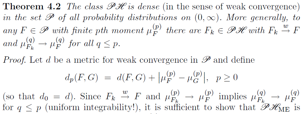
S. Asmussen (2003), Applied Probability and Queues, 2nd Edition, Springer
Class of phase-types is dense


p = 1
\text{Target}
p = 10
p = 25
p = 50
p = 100
p = 150
p = 200
p = 250
p = 300
Why does that work?
\tau_n \sim \mathrm{Erlang}(n, n/T) \,, \quad \tau_n \approx T
Can make a phase-type look like a constant value


f(s) = \boldsymbol{\alpha}^\top \mathrm{e}^{\boldsymbol{T} s} \boldsymbol{t}
How to fit them?
\mathrm{e}^{\boldsymbol{T} s} = \sum_{i=0}^\infty \frac{(\boldsymbol{T} s)^i}{i!}
\boldsymbol{\tau} = [\tau_1, \tau_2, \dots, \tau_n]
Observations:
L( \boldsymbol{\alpha} , \boldsymbol{T} \mid \boldsymbol{\tau} )
= \prod_{i=1}^n \boldsymbol{\alpha}^\top \mathrm{e}^{\boldsymbol{T} \tau_i} \boldsymbol{t}
Derivatives?
\ell( \boldsymbol{\alpha} , \boldsymbol{T} \mid \boldsymbol{\tau} ) = \sum_{i=1}^n \log\Bigl\{ \boldsymbol{\alpha}^\top \left[ \sum_{j=0}^\infty \frac{(\boldsymbol{T} \tau_i)^j}{j!} \right] \boldsymbol{t} \Bigr\}
Model (p.d.f.):
How to fit them?
\begin{aligned}
L( \boldsymbol{\alpha} , \boldsymbol{T} \mid \boldsymbol{B}, \boldsymbol{Z}, \boldsymbol{N} )
&= \prod_{i=1}^p \alpha_i^{B_i} \prod_{i=1}^p \mathrm{e}^{-t_{ii} Z_i } \prod_{i,j \text{ combs}} t_{ij}^{N_{ij}} \\
\end{aligned}
Hidden values:
\(B_i\) number of MC's starting in state \(i\)
\(Z_i\) total time spend in state \(i\)
\(N_{ij}\) number of transitions from state \(i\) to \(j\)
\boldsymbol{T} = \begin{bmatrix}
-t_{11} & t_{12} & t_{13} \\
t_{21} & -t_{22} & t_{23} \\
t_{31} & t_{32} & -t_{33}
\end{bmatrix}
\widehat{\alpha}_i = \frac{B_i}{n}
\widehat{t}_{i} = \frac{N_{i\dagger}}{Z_i}
\boldsymbol{t} = \begin{bmatrix}
t_1 \\
t_2 \\
t_3
\end{bmatrix}
\boldsymbol{\alpha} = \begin{bmatrix}
\alpha_1 \\
\alpha_2 \\
\alpha_3
\end{bmatrix}
\widehat{t}_{ij} = \frac{N_{ij}}{Z_i}
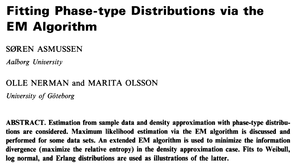
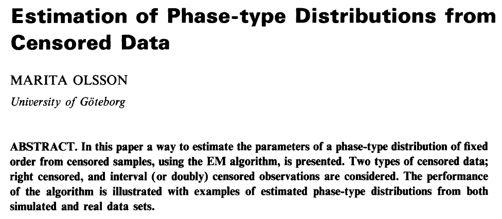
Diving into the source
c(y ; i \mid \alpha, T) = \int_0^y \alpha^\top \mathrm{e}^{T u} e_i \cdot \mathrm{e}^{T (y-u)} t \,\, \mathrm{d} u
i = 1, \dots, p
- Single threaded
- Homegrown matrix handling (e.g. all dense)
- Computational "E" step
- Instead solve a large system of DEs
- Hard to read or modify (e.g. random function)
c'(y ; i \mid \alpha, T) = T c(y ; i \mid \alpha, T) + [ \alpha^ \top \mathrm{e}^{T y} ]_i t
p(p+2)
C to Julia
void rungekutta(int p, double *avector, double *gvector, double *bvector,
		double **cmatrix, double dt, double h, double **T, double *t,
		double **ka, double **kg, double **kb, double ***kc)
{
  int i, j, k, m;
  double eps, h2, sum;

  i = dt/h;
  h2 = dt/(i+1);
  init_matrix(ka, 4, p);
  init_matrix(kb, 4, p);
  init_3dimmatrix(kc, 4, p, p);
  if (kg != NULL)
    init_matrix(kg, 4, p);
    ...
    for (i=0; i < p; i++) {
      avector[i] += (ka[0][i]+2*ka[1][i]+2*ka[2][i]+ka[3][i])/6;
      bvector[i] += (kb[0][i]+2*kb[1][i]+2*kb[2][i]+kb[3][i])/6;
      for (j=0; j < p; j++)
        cmatrix[i][j] +=(kc[0][i][j]+2*kc[1][i][j]+2*kc[2][i][j]+kc[3][i][j])/6;
    }
  }
}
This function: 116 lines of C, built-in to Julia
Whole program: 1700 lines of C, 300 lines of Julia
# Run the ODE solver.
u0 = zeros(p*p)
pf = ParameterizedFunction(ode_observations!, fit)
prob = ODEProblem(pf, u0, (0.0, maximum(s.obs)))
sol = solve(prob, OwrenZen5())
https://github.com/Pat-Laub/EMpht.jl

Lots of parameters to fit
- General
- Coxian distribution
\boldsymbol{\alpha} = \begin{bmatrix}
1 \\
0 \\
0
\end{bmatrix} , \quad
\boldsymbol{T} = \begin{bmatrix}
-t_{11} & t_{12} & 0 \\
0 & -t_{22} & t_{23} \\
0 & 0 & -t_{33}
\end{bmatrix} , \quad
\boldsymbol{t} = \begin{bmatrix}
t_1 \\
t_2 \\
t_{33}
\end{bmatrix}
\boldsymbol{\alpha} = \begin{bmatrix}
\alpha_1 \\
\alpha_2 \\
\alpha_3
\end{bmatrix} , \quad
\boldsymbol{T} = \begin{bmatrix}
-t_{11} & t_{12} & t_{13} \\
t_{21} & -t_{22} & t_{23} \\
t_{31} & t_{32} & -t_{33}
\end{bmatrix} , \quad
\boldsymbol{t} = \begin{bmatrix}
t_1 \\
t_2 \\
t_3
\end{bmatrix}
p^2 + (p-1)
p + (p-1)
In general, representation is not unique
A twist on the Coxian form
Canonical form 1
t_{11} < t_{22} < \dots < t_{pp}
\boldsymbol{\alpha} = \begin{bmatrix}
\alpha_1 \\
\alpha_2 \\
\alpha_3
\end{bmatrix} , \quad
\boldsymbol{T} = \begin{bmatrix}
-t_{11} & t_{11} & 0 \\
0 & -t_{22} & t_{22} \\
0 & 0 & -t_{33}
\end{bmatrix} , \quad
\boldsymbol{t} = \begin{bmatrix}
0 \\
0 \\
t_{33}
\end{bmatrix}
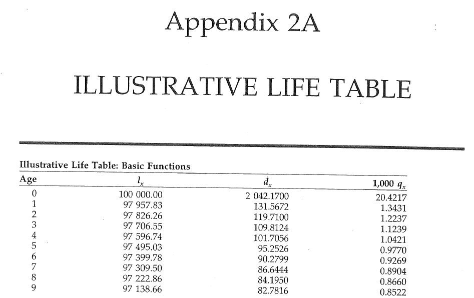
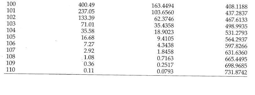
Problem: to model mortality via phase-type
Bowers et al (1997), Actuarial Mathematics, 2nd Edition
Final fit

p = 200
\text{Life Table}
using EMpht
lt = EMpht.parse_settings("life_table.json")[1]
phCF200 = empht(lt, p=200, ph_structure="CanonicalForm1")
Another cool thing
\mathbb{E}[ \mathrm{e}^{-\delta (\tau \wedge T) } \Psi(\overline{S}_{\tau \wedge T}, S_{\tau \wedge T}) ]
Contract over a limited horizon
Can use Erlangization so
\tau_n \approx T \,, \quad \tau_n \sim \mathrm{Erlang}(n, n/T)
\tau \wedge \tau_n = \tau_n^* \sim \mathrm{PhaseType}(\dots, \dots)
\ldots \approx \mathbb{E}[ \mathrm{e}^{-\delta \tau_n^* } \Psi(\overline{S}_{\tau_n^*}, S_{\tau_n^*}) ]
and phase-type closure under minimums
A. Vuorinen, The blockchain propagation process: a machine learning and matrix analytic approach
Phase-type for bitcoin
Heavy-tailed modeling?
Phase-types are always light-tailed

Can 'splice' together a Franken-distribution
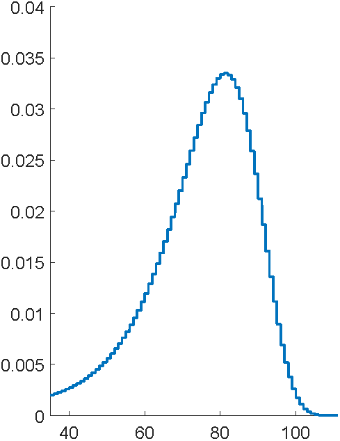
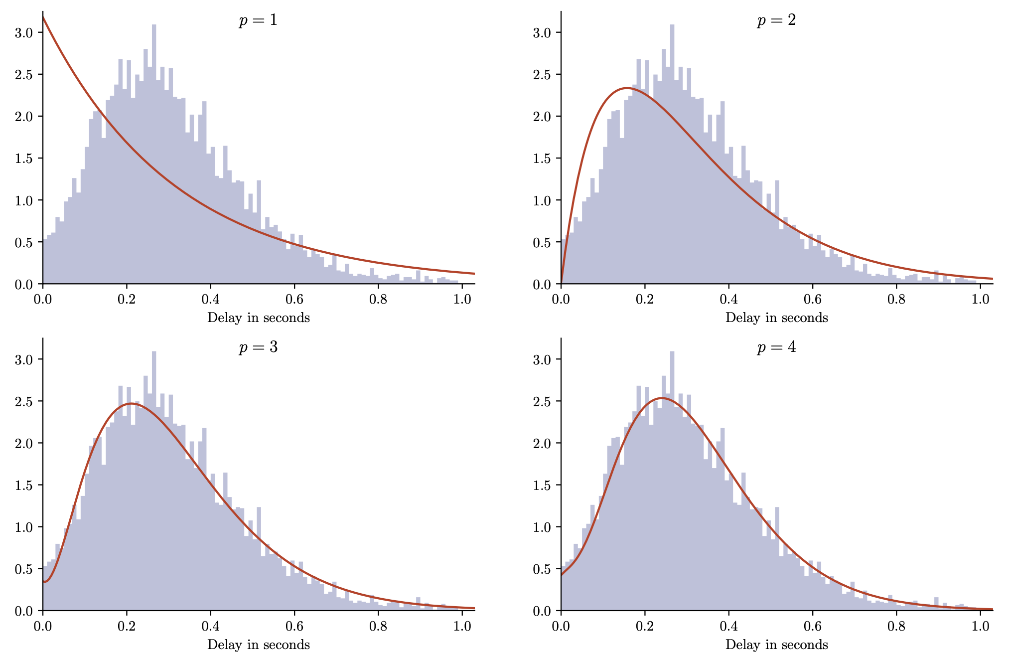
Norwegian fire data


Take logarithms

\tau_i = \log( X_i ) \sim \mathrm{PhaseType}(\boldsymbol{\alpha}, \boldsymbol{T}
)
Take logarithms and shift
\tau_i = \log( X_i ) - c \sim \mathrm{PhaseType}(\boldsymbol{\alpha}, \boldsymbol{T}
)
logClaims = log.(claims)
logClaimsCentered = logClaims .- minimum(logClaims) .+ 1e-4

~, int, intweight = bin_observations(logClaimsCentered, 500)
sInt = EMpht.Sample(int=int, intweight=intweight)

ph = empht(sInt, p=5)

logClaims = log.(claims)
logClaimsCentered = logClaims .- minimum(logClaims) .+ 1e-4

~, int, intweight = bin_observations(logClaimsCentered, 500)
sInt = EMpht.Sample(int=int, intweight=intweight)

ph = empht(sInt, p=40)
Take logarithms and shift
\tau_i = \log( X_i ) - c \sim \mathrm{PhaseType}(\boldsymbol{\alpha}, \boldsymbol{T}
)

Albrecher and Bladt, Inhomogeneous phase-type distributions and heavy tails, Journal of Applied Probability
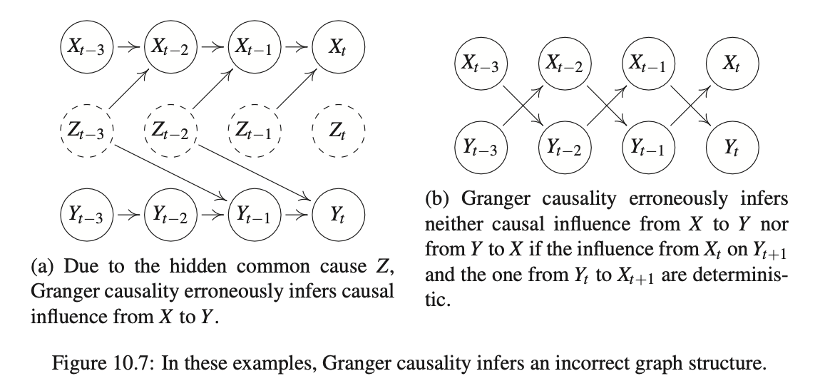
Causal analysis

Crime and temperature in Chicago
Empirical dynamic modelling
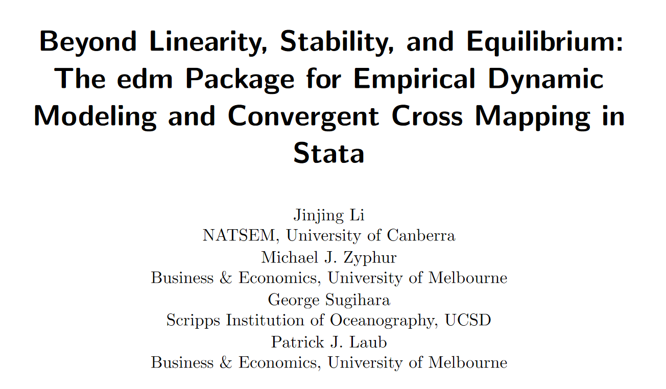
Quick Demo


Richard McElreath, Science as Amateur Software Development

Current projects
- EDM
- Missing data
- Alternative distance functions
- Hawkes process loss model with discounting
- Bayesian-model based (Rubin) causal inference for count data
Phase-type models in life insurance and empirical dynamic modelling
By plaub


