Dual-symmetric Electromagnetism:
A Clifford-algebraic approach
Justin Dressel
Schmid College of Science and Technology
Institute for Quantum Studies
Chapman University
Advances in Operator Theory
with Applications to Mathematical Physics
November 12-16, 2018, Chapman U, Orange CA
Physical Assumption : Minkowski Metric
-
Events can be locally described by a Minkowski pseudo-metric space (+,-,-,-)
- Local velocities (tangent vectors of curves that connect events) must be 4-vectors that obey this metric, according to observed Lorentz symmetries
- Connecting locally flat tangent spaces constructs an event-history manifold
- Local velocities (tangent vectors of curves that connect events) must be 4-vectors that obey this metric, according to observed Lorentz symmetries
-
Idea : Construct associative algebra that encodes the metric as a vector contraction
- Yields: (orthogonal) Clifford algebra \(\text{Cl}_{1,3}(\mathbb{R})\) ("Spacetime algebra")
as full geometric tangent space of the event-history manifold
- Nested Subalgebras (with natural physical meaning):
Clifford algebra \(\text{Cl}_{3,0}(\mathbb{R})\) (3D space relative to reference frame)
Quaternions \(\mathbb{H}\) (Rotation planes in 3D space)
Complex numbers \(\mathbb{C}\) (Single rotation plane)
Real numbers \(\mathbb{R}\) (Measurable quantity)
- Nested Subalgebras (with natural physical meaning):
- Yields: (orthogonal) Clifford algebra \(\text{Cl}_{1,3}(\mathbb{R})\) ("Spacetime algebra")
Constructing Spacetime Algebra
\text{Basis: } \gamma_0,\,\gamma_1,\,\gamma_2,\,\gamma_3
Minkowski Space \(\mathcal{M}_{1,3}(\mathbb{R})\) :
\displaystyle \begin{aligned}\eta(a+b,\,a+b) &= (a+b)^2 = a^2 + b^2 + ab + ba \\ &= \eta(a,a) + \eta(b,b) + 2\eta(a,b) \\ \implies& \eta(a,b) \equiv \frac{ab + ba}{2} \equiv a\cdot b \end{aligned}
\gamma_0 \cdot \gamma_0 = 1
\gamma_k \cdot \gamma_k = -1
\gamma_\mu \cdot \gamma_\nu = \eta_{\mu\nu} = \eta(\gamma_\mu,\,\gamma_\nu)
Minkowski metric
(symmetric bilinear form)
Algebraic Axioms: \(a,b,c\in\mathcal{M}_{1,3}(\mathbb{R})\)
- Associativity
\(a(bc) = (ab)c\)
- Left Distributivity
\(a(b+c) = ab + ac\)
- Right Distributivity
\((b+c)a = ba + ca\)
- Contraction
\(a^2 = aa = \eta(a,\,a)\)
Axioms constructively define Clifford algebra \( \text{Cl}_{1,3}(\mathbb{R}) \)
\displaystyle ab = \frac{ab + ba}{2} + \frac{ab - ba}{2} \equiv a\cdot b + a\wedge b
Symmetric part of product encodes metric:
Anti-symmetric part is Grassman wedge product:
(others zero)
Graded Clifford Basis
- Basis properties:
\gamma_0\gamma_1\gamma_2\gamma_3
\gamma_1\gamma_0 \quad \gamma_2\gamma_0 \quad \gamma_3\gamma_0 \quad | \quad \gamma_1\gamma_2 \quad \gamma_2\gamma_3 \quad \gamma_3\gamma_1
\gamma_0 \quad | \quad \gamma_1 \quad \gamma_2 \quad \gamma_3
1
Grade
0
1
2
3
\gamma_\mu\gamma_\nu = \begin{cases}-\gamma_\nu\gamma_\mu, & \mu\neq\nu \\ \eta_{\mu\nu}, & \mu = \nu \end{cases}
4
\gamma_1\gamma_2\gamma_3 \quad | \quad \gamma_0\gamma_2\gamma_3 \quad \gamma_0\gamma_1\gamma_3 \quad \gamma_0\gamma_1\gamma_2
2^4 = 16\;\text{elements}
Bivector Planes (of rotation):
3 hyperbolic | 3 elliptic
Vector Lines (of translation):
1 timelike | 3 spacelike
Scalar Points
Pseudovector Volumes:
1 spacelike | 3 timelike
Pseudoscalar 4-Volumes
Multivector: \( M = \langle M \rangle_0 + \langle M \rangle_1 + \langle M \rangle_2 + \langle M \rangle_3 + \langle M \rangle_4 \)
- Reciprocal basis:
\gamma^\mu \equiv (\gamma_\mu)^{-1} = \gamma_\mu / (\gamma_\mu)^2
Notational Simplifications
I
\vec{\sigma}_1 \quad \vec{\sigma}_2 \quad \vec{\sigma}_3 \quad | \quad I\vec{\sigma}_1 \quad I\vec{\sigma}_2 \quad I\vec{\sigma}_3
\gamma_0 \quad | \quad \gamma_1 \quad \gamma_2 \quad \gamma_3
1
0
1
2
3
I \equiv \gamma_0\gamma_1\gamma_2\gamma_3 \equiv \vec{\sigma}_1\vec{\sigma}_2\vec{\sigma}_3
(Spacetime-aware "imaginary unit" is the unit pseudoscalar: \(I^2 = -1\))
(commutes with even grade, anti-commutes with odd grade)
4
I\gamma_0 \quad | \quad I\gamma_1 \quad I\gamma_2 \quad I\gamma_3
Relative 3D space embedded as even-graded subspace:
\( \text{Cl}_{3,0}(\mathbb{R}) \)
Complexified 3-vector algebra is equivalent to this relative 3D Clifford algebra since \(I\) commutes with even grades
\vec{\sigma}_k \equiv \gamma_k\gamma_0 = \gamma_k \wedge \gamma_0
(Observed spatial directions in reference frame)
(Space axis dragged along temporal worldline)
Note duality transformation of left multiplication by \(-I\) : Hodge star operation
Multivector: \( M = [\alpha + (v_0 + \vec{v})\gamma_0 + \vec{A}] + I[\vec{B} + (w_0 + \vec{w})\gamma_0 + \beta] \)
Complex Structure & Spacetime Splits
Proper Form of Multivector:
\( M = \alpha + v + \mathbf{F} + Iw + I\beta = (\alpha + I\beta) + (v + Iw) + \mathbf{F} \)
Relative Frame Form of Multivector:
\( M = \alpha + (v_0 + \vec{v})\gamma_0 + (\vec{A} + I\vec{B}) + I(w_0 + \vec{w})\gamma_0 + I\beta \)
Components:
complex scalar
complex vector
bivector
scalar
polar paravector
polar vector
axial vector
axial paravector
pseudoscalar
4-vector
scalar
bivector
pseudovector
pseudoscalar
v = \sum_\mu v^\mu\gamma_\mu = \sum_\mu v_\mu \gamma^\mu = v_0 \gamma^0 + \sum_k v^k\vec{\sigma}_k\gamma_0
\mathbf{F} = \sum_{\mu,\nu} F^{\mu\nu}\gamma_\mu\gamma_\nu = \sum_{\mu,\nu} F_{\mu\nu} \gamma^\mu\gamma^\nu = \sum_k A^k\vec{\sigma}_k + I\sum_k B^k\vec{\sigma}_k
4-vector components, or a scalar and a relative 3-vector
rank-2 antisymmetric tensor components, or a pair of 3-vectors (one polar, one axial)
Fields and Derivatives
Multivector field: (in tangent algebra at point \(x\) of manifold)
\( M(x) = \alpha(x) + v(x) + \mathbf{F}(x) + Iw(x) + I\beta(x) \)
Vector derivative (Dirac operator):
\( \displaystyle \vec{\nabla} \equiv \sum_k \vec{\sigma}^k \frac{\partial}{\partial x^k} \) ; \( \vec{\nabla}\vec{v} = \vec{\nabla}\cdot\vec{v} + \vec{\nabla} \wedge \vec{v} = \vec{\nabla}\cdot\vec{v} + (\vec{\nabla}\times \vec{v})I \) (contains divergence and curl)
\(\nabla^2 = \nabla\gamma_0^2\nabla = (\partial_{ct} - \vec{\nabla})(\partial_{ct} + \vec{\nabla}) = \partial^2_{ct} - \vec{\nabla}\cdot\vec{\nabla} = \Box \) (d'Alembertian)
\displaystyle \nabla \equiv \sum_\mu \gamma^\mu \frac{\partial}{\partial x^\mu} = \gamma_0 \left[\frac{\partial}{\partial (ct)} + \vec{\nabla} \right] = \left[ \frac{\partial}{\partial (ct)} - \vec{\nabla} \right] \gamma_0
Physical Grade Examples
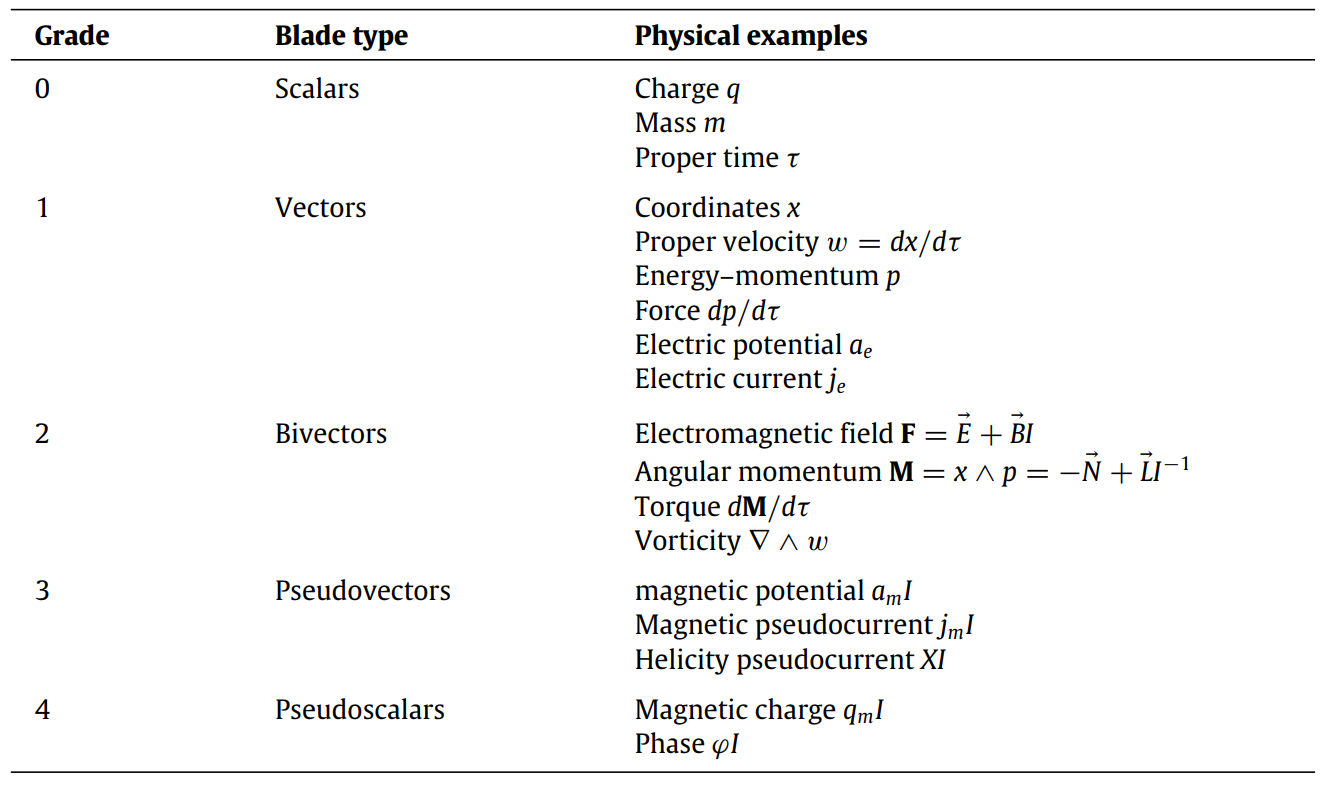
EM is naturally a bivector field
Maxwell's Equation
\mathbf{F}(x) = \sqrt{\epsilon_0}\left[\sum_{k=1}^3 E^k(x)\gamma_k\gamma_0 + Ic\sum_{k=1}^3 B^k(x) \gamma_k\gamma_0\right] = \sqrt{\epsilon_0}\vec{E}(x)+I\vec{B}(x)/\sqrt{\mu_0}
\nabla \mathbf{F} = j
j = \sum_\mu j^\mu_e \gamma_\mu + \sum_\mu j^{\mu}_{m} \gamma_\mu I = j_e + j_m I = \sqrt{\epsilon_0}(\rho_e + \vec{J}_e/c)\gamma_0 + \sqrt{\mu_0}(\rho_m + \vec{J}_m/c)\gamma_0 I
electric charge
density and current
This is Maxwell's Equation
\nabla F = \gamma_0(\vec{\nabla}\cdot\vec{E} + \partial_{ct}\vec{E}- \vec{\nabla}\times\vec{B}) + \gamma_0(\vec{\nabla}\cdot\vec{B} + \partial_{ct}\vec{B} + \vec{\nabla}\times\vec{E})I = \gamma_0(\rho_e - \vec{J}_e) + \gamma_0 (\rho_m - \vec{J}_m)I = j
Electromagnetic field bivector:
Same form as complex (Riemann-Silberstein) 3-vector
Electromagnetic source complex vector:
magnetic charge
density and current
Contains all of the usual 3D Maxwell's Equations, permitting both electric and magnetic charges
Canonical Field Decomposition and Phase
\mathbf{F}(x) = \sqrt{\epsilon_0}\vec{E}(x)+I\vec{B}(x)/\sqrt{\mu_0} = \mathbf{f}(x)\,e^{I\theta(x)/2}
\mathbf{f}^2 = |\mathbf{F}|^2 \geq 0
\mathbf{F}^2 = \left[\epsilon_0|\vec{E}|^2 - |\vec{B}|^2/\mu_0\right] + 2\sqrt{\epsilon_0/\mu_0}\,(\vec{E}\cdot\vec{B})I \equiv \ell_1 + \ell_2 I = |\mathbf{f}|^2 e^{I\theta}
Usual Lagrangian density for field
"axion" contribution to Lagrangian
Only possible Lorentz-invariant scalars
\mathbf{f}^2 = |\mathbf{F}|^2 = \sqrt{|\ell_1|^2 + |\ell_2|^2}
\displaystyle \theta = \tan^{-1}\frac{\ell_2}{\ell_1}
Note that a global phase degeneracy appears for a "null field" with zero magnitude
Null Solutions : Electromagnetic Waves
\mathbf{F}(x) = \sqrt{\epsilon_0}\vec{E}(x)+I\vec{B}(x)/\sqrt{\mu_0} = \mathbf{f}(x)\,e^{I\theta(x)/2}
\mathbf{f}^2 = |\mathbf{F}|^2 = 0
Even though null fields have global phase degeneracy, their local phases must be connected in order to satisfy Maxwell's equation, which breaks the phase symmetry
\mathbf{F}(x) = \mathbf{f}\,\exp[I\phi(x)]
Consider field with constant amplitude:
\nabla\mathbf{F} = 0 \implies [\nabla\phi]\mathbf{f} = 0
For phase and amplitude to both be nonzero, they must be noninvertible and therefore null
Since \(\mathbf{f}\) is constant, \(\nabla \phi\) must also be constant, which forces the linear solution :
\(\phi(x) = \phi_0 \pm k\cdot x \) with null wavevector \( k = \nabla \phi \),
as well as the decomposition \(\mathbf{f} = s\wedge k = -k\wedge s \) for some constant spacelike vector \(s\) s.t. \(s\cdot k = 0\)
Since the global phase is arbitrary, we choose \(\phi_0 = 0\) to find the plane-wave solutions:
\( \mathbf{F}(x) = sk\,e^{\pm I k\cdot x} \)
Writing out the directional null factor \(k = (\omega/c)\gamma_0(1 - \vec{k}/|\vec{k}|)\) and \(s = \vec{E}\gamma_0 \), this solution expands to:
\( \mathbf{F}(t,\vec{x}) = [\vec{E} \cos(\vec{k}\cdot\vec{x} - \omega t) \mp \hat{k}\times\vec{E} \sin(\vec{k}\cdot\vec{x} - \omega t)] + [\vec{E} \sin(\vec{k}\cdot\vec{x}-\omega t) \pm \hat{k}\times\vec{E} \cos(\vec{k}\cdot{x} - \omega t)]I \)
These are circularly polarized (constant helicity) electromagnetic plane wave modes.
Dual-symmetry : Electric-Magnetic Egalitarianism
\mathbf{F}(x) = \mathbf{f}(x)\,e^{I\theta(x)/2} = \sqrt{\epsilon_0}\vec{E}(x)+I\vec{B}(x)/\sqrt{\mu_0}
\nabla \mathbf{F} = j
j = j_e + j_m I = \sqrt{\epsilon_0}(\rho_e + \vec{J}_e/c)\gamma_0 + \sqrt{\mu_0}(\rho_m + \vec{J}_m/c)\gamma_0 I
\(\{\)
Complete EM dynamics:
A hidden gauge symmetry is now evident:
e^{-I\phi/2}\nabla \mathbf{F}e^{I\phi/2} = e^{-I\phi/2}je^{I\phi/2}
The pseudoscalar \(I\) generates phase rotations in the usual way:
this has the effect of swapping the electromagnetic fields and source charges
e^{-I\phi/2}\nabla \mathbf{F}e^{I\phi/2} = \nabla\left[e^{I\phi/2}\mathbf{F}e^{I\phi/2}\right] = \nabla \left[\mathbf{F}e^{I\phi}\right] = \nabla \left[ (\cos\phi\,\vec{E} - \sin\phi\,\vec{B}) + (\sin\phi\,\vec{E} + \cos\phi\,\vec{B})I\right] = \nabla(\vec{E}' + \vec{B}'I)
e^{-I\phi/2}je^{I\phi/2} = je^{I\phi} = (\cos\phi\,j_e - \sin\phi\,j_m) + (\sin\phi\,j_e + \cos\phi\,j_m)I = j_e' + j_m'I
Physics is the same provided that both source and field definitions are changed in tandem
Can always choose \(\phi\) to make all charges electric (\(j'_m = 0\))
Vacuum fields (\(j = 0\)) always have this field-exchange symmetry
Electromagnetic Vector Potentials
\mathbf{F}(x) = \nabla z(x)
Postulate vector potential:
z(x) = a_e(x) + a_m(x)I
Must be complex field to satisfy dual symmetry
\mathbf{F} = \mathbf{F}_e + \mathbf{F}_m I = \nabla \wedge a_e + (\nabla\wedge a_m)I
0 = \nabla \cdot a_e = \nabla\cdot a_m
Lorenz-Fitzgerald conditions assumed
\mathbf{F} = \vec{E} + \vec{B}I ; \qquad a_e = (\phi_e + \vec{A})\gamma_0 ; \qquad a_m = (\phi_m + \vec{C})\gamma_0
\vec{E} = -\vec{\nabla}\phi_e - \partial_{ct}\vec{A} - \vec{\nabla}\times\vec{C}
\vec{B} = -\vec{\nabla}\phi_m - \partial_{ct}\vec{C} + \vec{\nabla}\times\vec{A}
Relative EM fields regain apparent symmetry in definitions
\implies \nabla\mathbf{F}(x) = \nabla^2 z(x) = j(x)
Obvious wave equation
Lorentz Force
\displaystyle \frac{dp}{d\tau} = \langle\mathbf{F}j\rangle_0 = q_e\,\mathbf{F}\cdot w + q_m (\mathbf{F}\wedge w)I
Proper force law:
p \equiv m w \qquad j \equiv q w \qquad q \equiv q_0\,e^{I\theta} = q_e + q_m I
Charge must be complex to admit dual symmetry
\displaystyle w \equiv \frac{dx}{d\tau} = \gamma(c + \vec{v})\gamma_0 \qquad w^2 = c^2 \qquad \gamma \equiv (1 - |\vec{v}/c|^2)^{-1/2}
\displaystyle \gamma c \equiv \frac{dt}{d\tau} = w\cdot\gamma_0 \qquad \gamma\vec{v} \equiv \frac{d\vec{x}}{d\tau} = w\wedge\gamma_0
\displaystyle \frac{dp}{d\tau}\frac{d\tau}{dt}\gamma_0 = \frac{d\mathcal{E}}{d(ct)} + \frac{d\vec{p}}{dt} \qquad \mathcal{E} \equiv \gamma mc^2 \qquad \vec{p} = m\vec{v} \qquad \frac{\vec{v}}{c} = \frac{w\wedge \gamma_0}{w\cdot\gamma_0}
Relative force law:
\displaystyle \frac{d\mathcal{E}}{d(ct)} = q_e \vec{E}\cdot\vec{v} + q_m \vec{B}\cdot \vec{v}
\displaystyle \frac{d\vec{p}}{dt} = q_e \vec{E} + q_m \vec{B} + q_e \vec{v}\times\vec{B} - q_m \vec{v}\times\vec{E}
Rate of work performed (c=1)
Relative Lorentz force, including magnetic charge
Noether's Theorem and Dual Symmetry
e^{-I\phi/2}\nabla \mathbf{F}e^{I\phi/2} = e^{-I\phi/2}je^{I\phi/2}
A new gauge symmetry leads to an independently conserved quantity : certainly conserved in vacuum
\underline{X}(I) = [\chi I + \vec{S}I^{-1}]\gamma_0
Helicity Pseudocurrent (tensor) is newly conserved
\chi = \vec{B}_e \cdot \vec{A} - \vec{E}_m \cdot \vec{C}
\vec{S} = \vec{E}_e\times\vec{A} + \vec{B}_m\times \vec{C}
Spin-density vector is the helicity flux density
Scalar helicity density
These definitions only make sense when full dual-symmetric fields are used
They match postulated definitions of these quantities in the constrained case with \( \mathbf{F} = \mathbf{F}I \)
Conclusions
- Spacetime Clifford algebra is the natural language of electromagnetism
- The dual-symmetric structure of the electromagnetic theory becomes manifest when expressed in geometrically invariant forms
- The conserved quantity from Noether's theorem resulting from the continuous dual-symmetry in vacuum field propagation is the helicity
- Dual-symmetry is spontaneously broken by the convention to make all charges electric. The symmetry is preserved if electric and magnetic charges are simultaneously swapped with the fields.
Thank you!
JD, et al. Physics Reports 589 1-71 (2015)
Dual-symmetric Electromagnetism, a Clifford-algebraic approach
By Justin Dressel
Dual-symmetric Electromagnetism, a Clifford-algebraic approach
Advances in Operator Theory with Applications to Mathematical Physics November 12-16 2018, Chapman University, ORANGE, CA Abstract: We show how to use Minkowski spacetime Clifford algebra to efficiently describe electromagnetism. The electric and magnetic fields are combined into a single complex and frame-independent bivector field, which generalizes the Riemann-Silberstein complex vector that has recently resurfaced in studies of the single photon wavefunction. The complex structure of spacetime also underpins the emergence of electromagnetic waves, circular polarizations, the normal variables for canonical quantization, the distinction between electric and magnetic charge, complex spinor representations of Lorentz transformations, and the dual (electric-magnetic field exchange) symmetry that produces helicity conservation in vacuum fields. This latter symmetry manifests as an arbitrary global phase of the complex field, motivating the use of a complex vector potential, along with an associated transverse and gauge-invariant bivector potential, as well as complex (bivector and scalar) Hertz potentials.


