Quantum Measurements
with Quasiprobabilities
Justin Dressel
Institute for Quantum Studies, Chapman University
QuiDiQua Conference, 2023/11/10
Classical Field Theory
How do we measure what the Electric Field is at some point \(x\) in space?
We put a "test charge" at \(x\) and look at its response.
Electric Field: \(\displaystyle \vec{E} \equiv \frac{\vec{F}}{q}\Bigg|_{q\to 0} \)
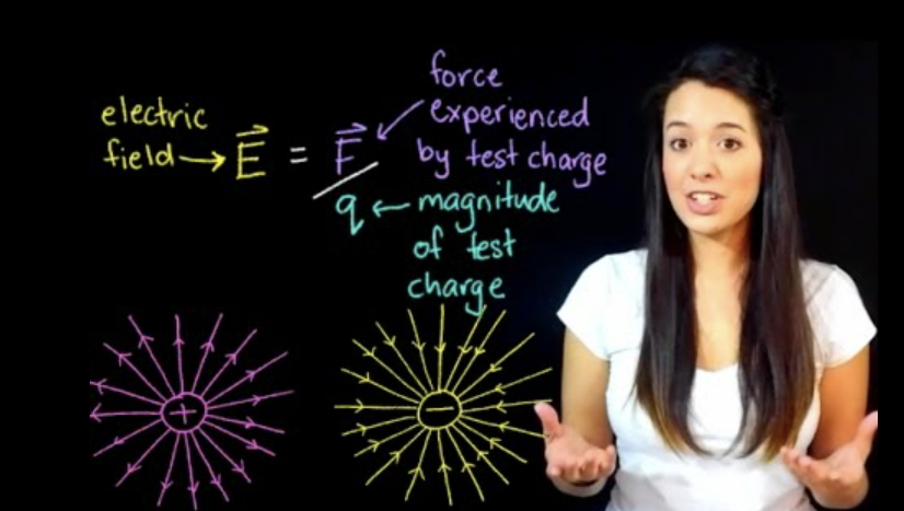
We take the weak interaction limit where the test charge is small, so the field we are measuring is not disturbed by the test charge itself.
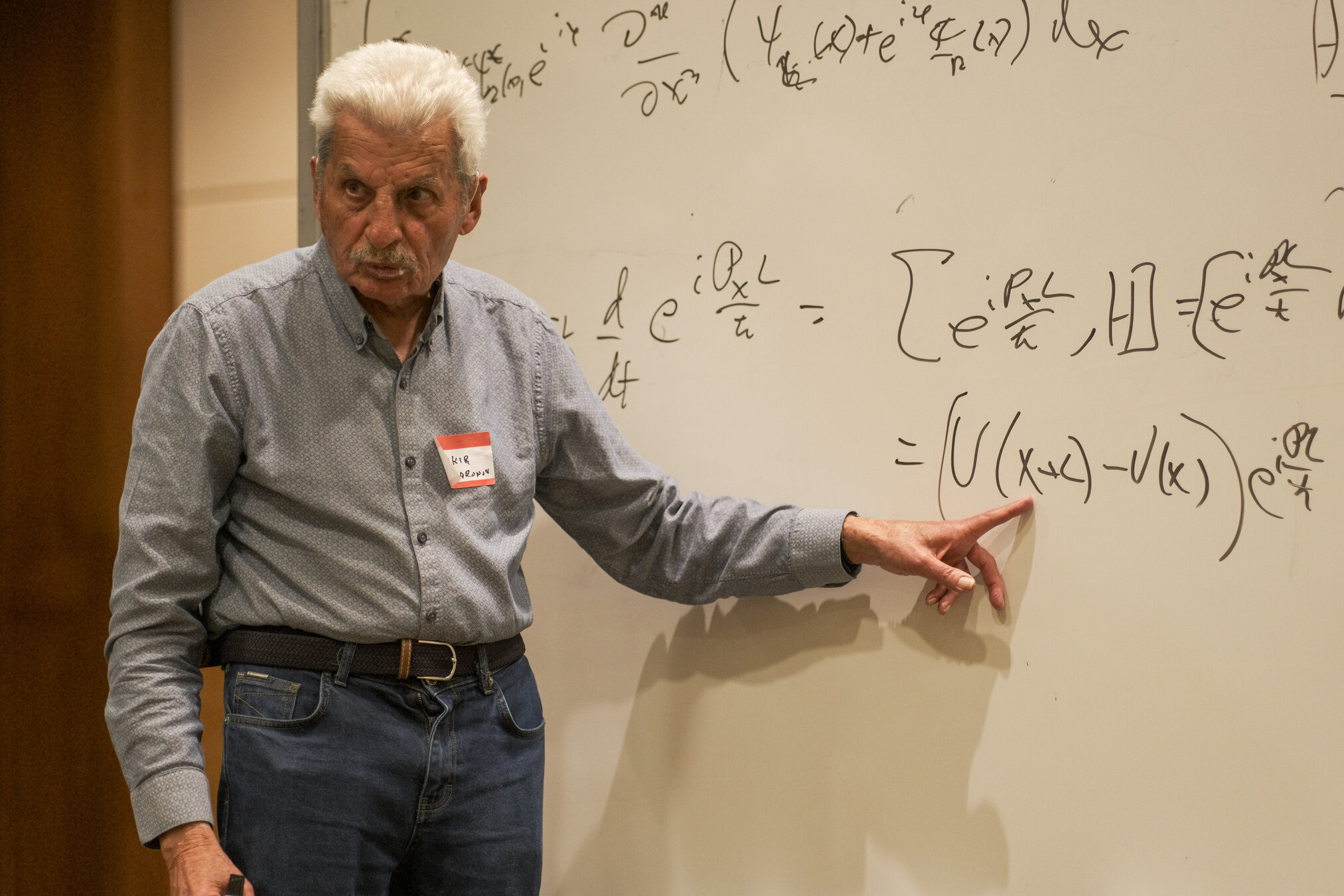
Quantum Theory
Yakir Aharonov:
"Let's do exactly the same thing with quantum theory."
Probe charge: \(|\phi\rangle\) s.t. \(\langle \hat{x}\rangle = 0\)
System: \(|\psi\rangle\)
Interaction: \(\hat{H} = q\hat{A}\otimes\hat{p}\)
Response:
\(e^{-iqt\hat{A}\hat{p}/\hbar}|\psi\rangle|\phi\rangle = \sum_a\int dx |a\rangle|x\rangle\, \langle a|\psi\rangle\,\langle x-qat|\phi\rangle \)
Mean velocity per charge yields:
\(\displaystyle \frac{\partial_t\langle \hat{x}\rangle}{q}\Bigg|_{q\to 0} = \sum_a |\langle a|\psi\rangle|^2 a = \langle \hat{A}\rangle \)
Expectation value of \(\hat{A}\) measured without probe disturbing the system (much).
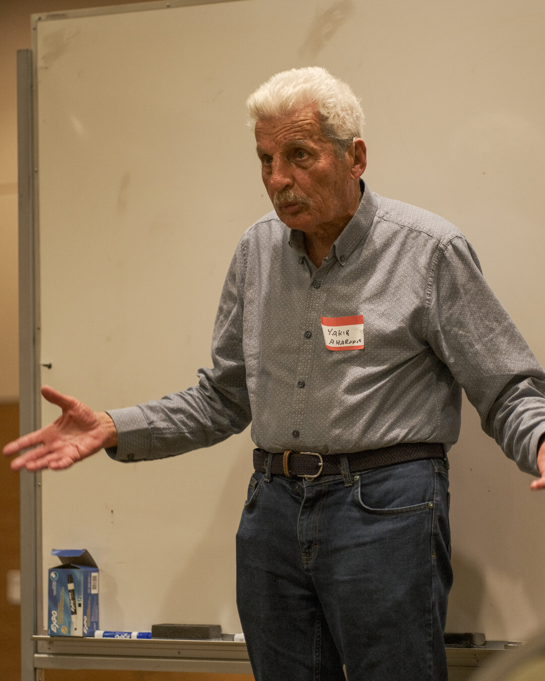
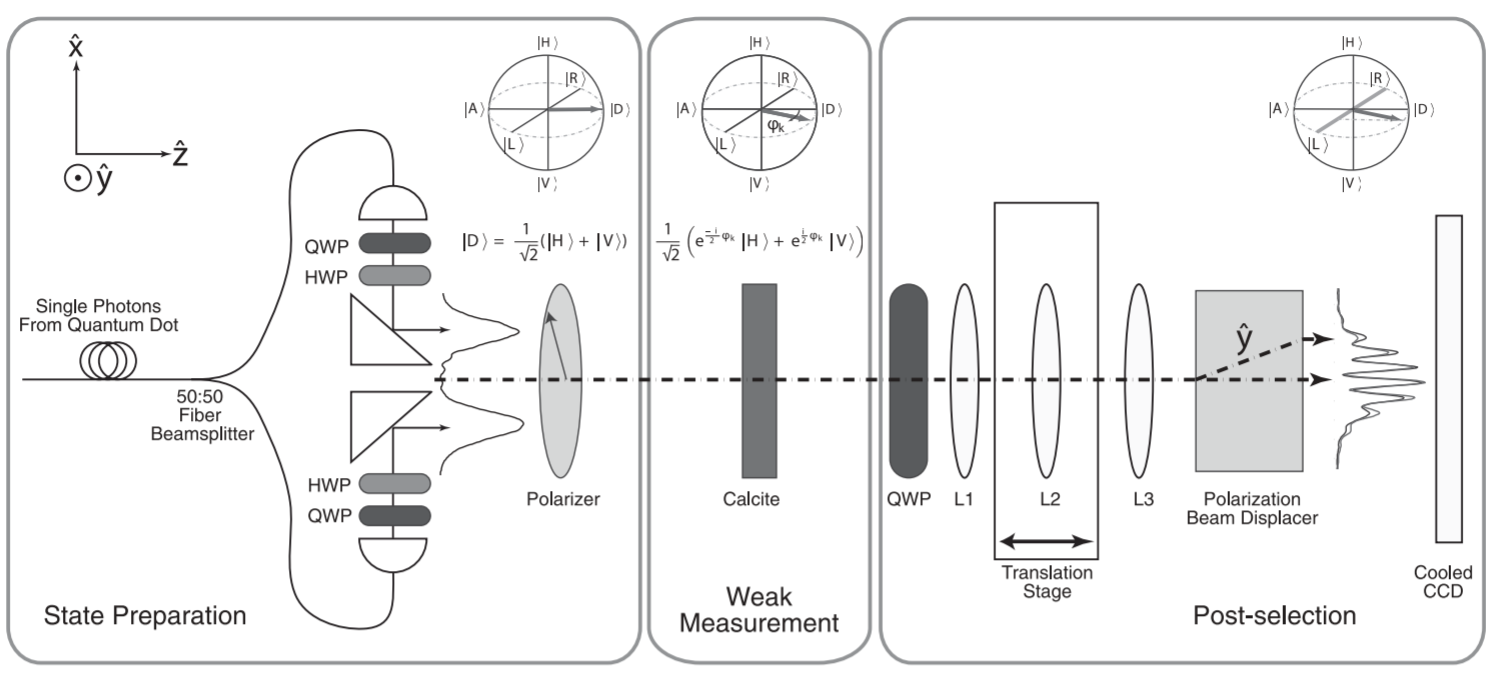
Postselecting Quantum Theory
Yakir Aharonov:
"Let's do exactly the same thing with quantum theory, but also add a final postselection measurement."
System Postselection: \(\langle f |\)
Small test charge response:
\(\begin{aligned}\langle f |e^{-iqt\hat{A}\hat{p}/\hbar}|\psi\rangle|\phi\rangle &\approx \langle f |\psi\rangle(1 -iqt A_w\hat{p}/\hbar)|\phi\rangle \\ &\approx \langle f|\psi\rangle \int dx |x\rangle\, \,\langle x-q A_w t|\phi\rangle \end{aligned}\)
Mean velocity per charge yields:
\(\displaystyle \frac{\partial_t\langle \hat{x}\rangle}{q}\Bigg|_{q\to 0} = \text{Re}A_w \equiv \text{Re} \frac{\langle f | \hat{A}|\psi\rangle}{\langle f | \psi \rangle} \)
The expectation value of \(\hat{A}\) conditioned on a final postselection \(\langle f|\) is a weak value.
Aharonov et al. PRL 1988
Weak Value:
A "conditioned expectation value" measured in the weak interaction ("test charge") limit.
\displaystyle A_w \equiv \frac{\langle f | \hat{A} | \psi \rangle}{\langle f | \psi \rangle} = \frac{\langle \psi | f\rangle\!\langle f | \hat{A} | \psi \rangle}{|\langle f | \psi \rangle|^2}
An expectation value is partitioned into a convex mixture of weak values,
each specific to a particular "postselection".
\displaystyle \langle A \rangle \equiv \langle \psi | \hat{A} | \psi \rangle = \sum_f \langle \psi | f \rangle\!\langle f |\hat{A} | \psi \rangle = \sum_f |\langle f | \psi \rangle|^2 \frac{\langle f | \hat{A} | \psi \rangle}{\langle f | \psi \rangle} = \sum_f P_{f|\psi}\, A_{w,f}
Weak values are not necessarily constrained by the spectrum of the operator \(\hat{A}\).
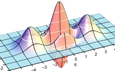
Kirkwood-Dirac Quasiprobabilities:
The "conditioned probabilities" that average the eigenvalues of \(\hat{A}\) are quasiprobabilities.
\displaystyle A_w \equiv \frac{\langle \psi | f\rangle\!\langle f | \hat{A} | \psi \rangle}{|\langle f | \psi \rangle|^2} = \sum_a a \frac{\langle \psi | f\rangle\!\langle f | a\rangle\!\langle a | \psi \rangle}{|\langle f | \psi \rangle|^2} = \sum_a a \frac{Q_{a,f|\psi}}{P_{f|\psi}}
The Kirkwood-Dirac quasiprobabilities are conditioned by the postselection likelihoods.
Q_{a,f|\psi} \equiv \langle \psi | f\rangle \!\langle f | a \rangle\!\langle a | \psi \rangle = |Q_{a,f|\psi}|\,e^{iS}
The phase is a geometric Berry/Pancharatnam phase determined by the
oriented area enclosed by geodesics connecting three quantum states.
Classically compatible states enclose zero area.
Non-zero phases encode dynamical incompatibility and a temporal directionality for closing the loop.
2\(S\)
\(|\psi\rangle\)
\(|a\rangle\)
\(|f\rangle\)
Hofmann, NJP 2011
Dynamical
Weak Values
Due to their close connection to the geometry of quantum state space, weak values (and thus the KD QP) can appear even without making any explicit weak measurements.
Let's explore several examples.
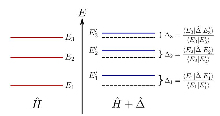
\hat{H}|E_k\rangle = E_k |E_k \rangle
(\hat{H}+\hat{\Delta})|E'_j\rangle = E'_j |E'_j \rangle
\langle E'_j |(\hat{H}+\hat{\Delta})|E_k\rangle = E'_j \langle E'_j | E_k \rangle = E_k \langle E'_j | E_k \rangle + \langle E'_j |\hat{\Delta}| E_k \rangle
\displaystyle E'_j - E_k = \frac{\langle E'_j | \hat{\Delta} | E_k \rangle}{\langle E'_j | E_k \rangle}
Measurable energy shifts caused by a perturbation are always (purely real) weak values.
"Strange weak values" outside the spectrum of the perturbation are very common.
JD, PRA 91 032116 (2015)
Trivial Example of Dynamical Weak Values:
When a perturbation is added to a Hamiltonian, the energy spectra will shift by weak values of the perturbation.
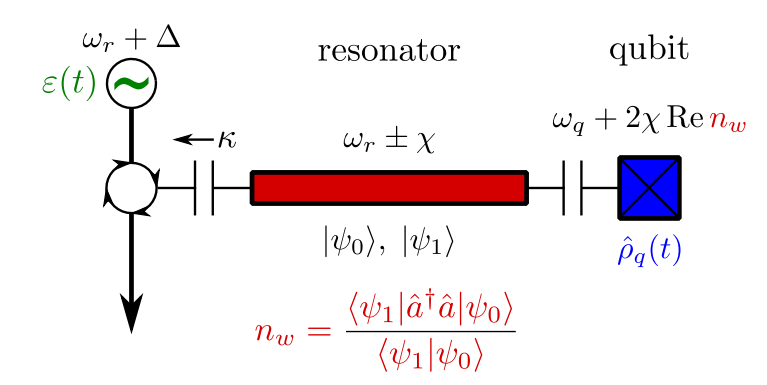
Nontrivial Example: Circuit QED
\displaystyle \hat{H} = \frac{\omega_q}{2}\hat{\sigma}_z + \omega_r \hat{a}^\dagger \hat{a} + \chi \hat{\sigma}_z \hat{a}^\dagger \hat{a}
At steady state, the balance of pump and decay from the resonator leaves the qubit entangled with distinct coherent states in the resonator:
Dispersive Coupling Hamiltonian:
|\Psi\rangle = c_0 |0\rangle |\psi_0\rangle + c_1 |1\rangle |\psi_1\rangle
This reduced state qubit coherence evolves as:
\rho_{01}(t) = c_1^* c_0 \langle \psi_1 | \psi_0\rangle
The coherence of the reduced qubit state is thus:
\partial_t \rho_{01}(t) = i[\omega_q + 2\chi \,n_w]\rho_{01}(t)
\displaystyle n_w \approx \frac{4\varepsilon^2}{\kappa^2}\left[1 + i\frac{4\chi}{\kappa}\right] \equiv \bar{n} + i\frac{4\chi \bar{n}}{\kappa}
Photon number weak value!
- Real part : AC Stark shift
- Imaginary part : ensemble dephasing
\Delta\omega_q = 2\chi\,\text{Re}\,n_w = 2\chi\bar{n}
\displaystyle \Gamma = 2\chi \,\text{Im}\,n_w = \frac{8\chi^2\bar{n}}{\kappa}
JD, PRA 91 032116 (2015)
For pump \(\varepsilon\) and decay rate \(\kappa\), the steady states yield:
\displaystyle i\hbar \partial_t |\psi(t)\rangle = \left[ \frac{\hat{p}^2}{2m} + V(\hat{x}) \right] |\psi(t)\rangle
Schrodinger Equation:
Hamilton's Principle Function :
S(t, x) \equiv -i\hbar \ln\langle x | \psi(t) \rangle
\displaystyle p_w(t,x) \equiv \partial_x S(t,x) = \frac{-i\hbar\partial_x\psi(t,x)}{\psi(t,x)} = \frac{\langle x | \hat{p} | \psi(t) \rangle}{\langle x | \psi(t) \rangle}
Momentum defined in the usual way is the weak value of the momentum operator:
Schrodinger's Equation is equivalent to a quantum Hamilton-Jacobi Equation:
\partial_t S(t, x) + H_w[t,x, p_w(t,x)] = 0
\displaystyle \text{Re} H_w[t,x, p(t,x)] = \frac{(\text{Re}\,p_w(t,x))^2}{2m} + V(x) + Q(x)
Imaginary part is a continuity equation for probability. Real part is classical HJ Equation:
\displaystyle Q(x) = \frac{\langle x| (\hat{p} - \text{Re}\,p_w(t,x))^2 | \psi(t) \rangle}{\langle x | \psi(t) \rangle} = -\frac{\hbar^2}{2m}\frac{\partial_x^2 |\psi(x,t)|}{|\psi(x,t)|}
"Quantum Potential": Weak Variance of momentum away from mean weak value
Nontrivial example: Hamilton-Jacobi Theory
\displaystyle H_w[t,x, p_w(t,x)] = \frac{\langle x | \hat{p}^2/2m + V(\hat{x}) | \psi \rangle}{\langle x | \psi \rangle}
Real part: Bohmian momentum
Imaginary part: Nelson Osmotic momentum
JD, PRA 91 032116 (2015)
Nontrivial example: Classical field streamlines
Weak values also appear as physical properties of a classical field, even when there is not an obvious "weak measurement" at the level of individual field quanta.
Momentum weak value proportional to the local (orbital part of the) Poynting vector \(S_O\) of an optical field, scaled by the frequency \(\omega\) and energy density \(W\).
This can be measured and used to reconstruct "averaged trajectories" for the mean momentum streamlines.
The average local momentum corresponds to the local optical pressure felt by small probe particles, and thus the momentum part of the stress-energy tensor.
Kocsis et al., Science (2011)
Bliokh et al. NJP (2013)
\displaystyle \text{Re}\,\mathbf{p}(\mathbf{r}) = \text{Re} \frac{\langle x | \hat{p} | \psi \rangle}{\langle x | \psi \rangle} = \frac{\omega}{c^2} \frac{S_o(\textbf{r})}{W(\textbf{r})}
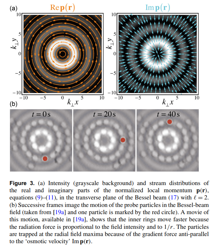
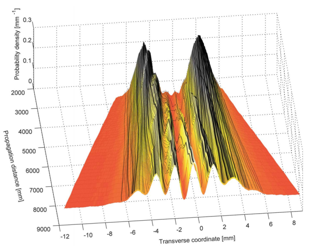
Nontrivial Example: Bessel beams
Both real and imaginary parts of this local momentum average also describe physical properties of classical "vortex beams" like Bessel beams.
\displaystyle \mathbf{p}_w(\mathbf{r}) = \frac{\langle x | \hat{p} | \psi \rangle}{\langle x | \psi \rangle}
The real part of the momentum weak value appears as the circulating local orbital momentum that can be transferred to probe particles by pushing them around in circular orbits.
The imaginary part is directed radially and confines the optical intensity into concentric rings, similarly trapping probe particles to orbit only within the optical rings.
Bliokh et al., NJP (2013)
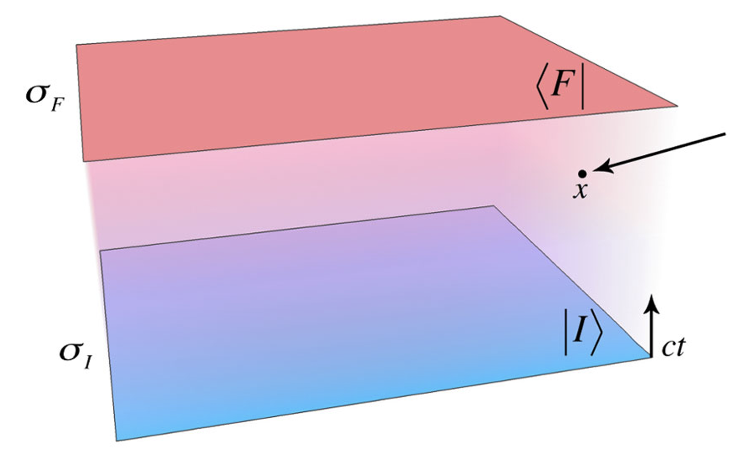
Quantum Field Theory
Boundary conditions:
- Past time \(t_I\): \(|I\rangle\)
- Future time \(t_F\): \(\langle F |\)
"Test charge" current:
- Intermediate time \(t\): \(J(x)\)
- Take limit as \(J \to 0\)
But wait, there's more!
Schwinger taught us to do exactly the same thing in quantum field theory to probe mean (classical) fields and their correlations
Schwinger, PR (1951)
QFT: Classical Mean Fields
Generating Functional:
\(W[J] = -i\hbar \ln\langle F |\hat{U}[J] | I \rangle \)
Effective Action:
\(\Gamma[\varphi] = W[J] - \int d^4x J(x)\varphi(x)\)
"Classical" Field:
\(\displaystyle \varphi(x) \equiv \frac{\delta W[J]}{\delta J(x)}\Bigg|_{J\to 0} \!\! = \frac{\langle F(t)|\hat{\varphi}(x)|I(t)\rangle}{\langle F(t)|I(t)\rangle}\)
"Classical" Equation of Motion:
\(\displaystyle \frac{\delta \Gamma[\varphi]}{\delta \varphi(x)} = -J(x) \to 0\)
All classical fields according to QFT are weak values of the field operators.
JD, PRL (2014)
Summary
Weak values are prevalent in the quantum formalism,
even without performing weak measurements,
which means that Kirkwood-Dirac quasiprobabilities are also!
- Conditioned average of weakly measured observable
- Spectral shifts due to perturbations
- Ensemble-averaged dynamical parameters
- Classical mean field properties
- Classical limit for observable values
- ...and many more examples
Thank you!
Quantum Measurements with Quasiprobabilities
By Justin Dressel
Quantum Measurements with Quasiprobabilities
Invited talk for the QuiDiQua conference, 2023/11/10


