Introduction to data analysis using machine learning
David Taylor, data scientist
prooffreader.com
dtdata.io
@prooffreader
Introduction to data analysis using machine learning
I made sure to put this in the title because it's not obvious from the name "Machine Learning" exactly what it does.
Goals of this presentation:
-
To demystify the field of machine learning (ML)
-
To introduce you to the vocabulary and fundamental concepts ("idea buckets") of ML
-
To serve as a foundation for further learning about ML
-
To provide links to further resources for self-learning about ML (including some IPython notebooks I made)
To see this presentation and handy links, go to:
http://www.dtdata.io/introml
There are two versions:
- "lite" (for live presentation)
- "complete" (for self-study)
All of the examples were made with Python using Scikit-Learn and Matplotlib
What is machine learning?

What is machine learning?
Don't worry, not this.

What is machine learning?
It is the use of algorithms to create knowledge from data.
What is machine learning?
It is the use of algorithms to create knowledge from data.
What's an algorithm?
What is machine learning?
It is the use of algorithms to create knowledge from data.
What's an algorithm?
A set of rules/instructions.
If A, then do B.
Then if C, do D, otherwise do E.
etc.
What is machine learning?
How many of you have done machine learning before?
What is machine learning?
How many of you have done machine learning before?
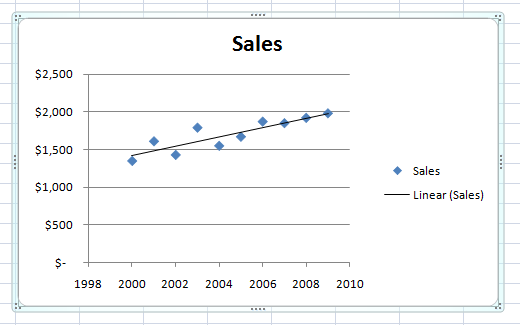
How many of you have made a best-fit linear regression line in Excel before?
What is machine learning?
How many of you have done machine learning before?
How many of you have made a best-fit linear regression line in Excel before?
If so, you've done machine learning. Best-fit regression uses an algorithm to minimize the sum of squared vertical distances from each point to the line
What is machine learning?
"But wait! All I did was push a button in Excel!"
You can do lots of machine learning in lots of platforms by just entering your data into a "black box" and getting the results without understanding the process at all.
(Of course, just like a best-fit regression line, if you don't understand the process, you're in danger of misinterpreting the results, especially if you "don't know what you don't know".)
What is machine learning?
Machine Learning is an offshoot of the field of Artifical Intelligence, born in the 1950s when extremely rapid scientific progress made many optimistic about the possibility that computers could achieve human-like intelligence in a matter of decades (many felt the same way about extraterrestial colonization as well).
As the scope of the challenges of AI became more clear, the field bifurcated into AI and ML, especially as ML applications to business intelligence (i.e. $$$) became clear in the 1980s.
AI still exists as a vigorous field of study,
but its expectations are more realistic now.
Examples of machine learning
Autocorrect
Google page ranking
Netflix suggestions
Credit card fraud detection
Stock trading systems
Climate modeling and weather forecasting
Facial recognition
Self-driving cars
Simple data analysis
A note on nomenclature
Much of the vocabulary in machine learning -- including the term "machine learning" itself -- have meanings that are somewhat askew from how these words are used outside the field, e.g. "supervised", "bias/variance", "precision/recall"
Why? A lot of the vocabulary dates from the 1950s; the first highly successful algorithm was named the Perceptron. It sounds like it's straight from an Isaac Asimov novel.
The Dataset
I invented a dataset based on a well-known
machine learning dataset about Italian wines.
Instead of wines, it is a dataset about fruit.
It allows you to ...
The Dataset
I invented a dataset based on a well-known
machine learning dataset about Italian wines.
Instead of wines, it is a dataset about fruit.
It allows you to ...
... wait for it ...
The Dataset
I invented a dataset based on a well-known
machine learning dataset about Italian wines.
Instead of wines, it is a dataset about fruit.
It allows you to ...
... wait for it ...
... compare apples and oranges!
The Dataset

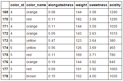
The Dataset
Color: a categorical variable, assigned an arbitrary numeric ID from 1-6.
I introduced "noise" by simulating color-blindedness in the observations,
e.g. green to red
The Dataset
Elongatedness:
0 = circular,
1=twice as long as wide,
infinite = line
The Dataset
Weight, sweetness and acidity are numerical measurements; we have "lost" the units, but that's okay, since we'll standardize everything.
Instances
Rows are called instances.
Each instance is a separate set of observations of one replicate of the subject of the dataset.
This dataset has 179 instances.
Features
Columns/Variables are called features.
They can be:
- Numeric
- Interval,
e.g. date or time - Ordinal
- Categorical
If I were collecting data about the people in this room, every person would be an instance.
What would be some features?
Numeric, Interval, Ordinal, Categorical?
Numerical, e.g. height
* any arithmetical operation can be performed, e.g. average
Interval, e.g. birthday
* can be subtracted only; 1992 - 1975 = 17 years,
but 1992 + 1975 is meaningless (arbitrary zero)
Ordinal, e.g. level of education completed
* Graduate school > Undergrad > High School, but no subtraction
Categorical, e.g. hair color
* can assign numbers for convenience only
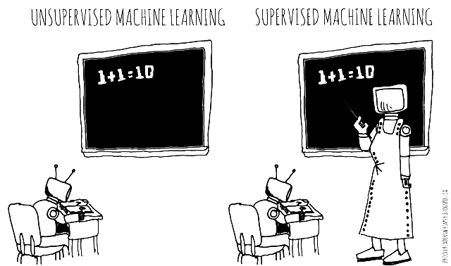
Two kinds of
machine learning:
Unsupervised
and Supervised
from my webcomic, prooffreaderswhimsy
Unsupervised = exploratory
Supervised = predictive
We'll hold off from further comparison of unsupervised and supervised learning for now;
We'll do some unsupervised learning first to give you some context.
Unsupervised learning is also known as "clustering".
We try to find "clusters" in which members of the cluster have more in common with each other than instances that are not in the cluster.
Let's do some
Unsupervised Machine Learning
of our fruit dataset
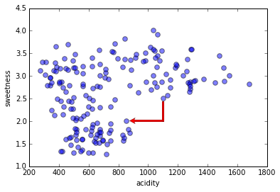
We will use only two of the five features of our dataset ("sweetness" and "acidity"), because it's a lot easier to visualize only two dimensions of numeric features, but clustering can be done on any number of dimensions with any kind of features.
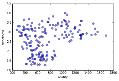
We are looking for clusters, i.e. sets of instances (data points) that are more similar to each other than to instances not in the set.
There is never an a priori number of clusters; every data point could be its own cluster, the entire dataset could be one cluster, and everything in between.
How many clusters
do you see?
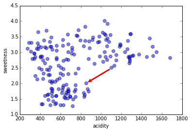
Another way to think of a cluster regions of
high density separated by regions of low density.
Another way to think of a cluster regions of
high density separated by regions of low density.
By defining what we mean by high and low density, we can have a "natural", i.e. intrinsic to the dataset, determination of how many clusters there are.
Density of what, exactly?
We need a distance function. (Sometimes we call it a 'similarity function'; similarity is the opposite of distance, but they measure the same thing.)
In this kind of plot, distance might be intuitive, but with other features such as categorical data, it can be a crucial decision that affects the outcome.
A common distance function for numeric data is Euclidian distance.
But the data must be normalized! Otherwise, in this case, acidity would have a much higher effect on the distance function than sweetness just because of its (arbitrary) units.
Here's another distance measure, "Manhattan distance" (named after city blocks in downtown New York City).
There are many distance functions you can use. Very often changing a distance function makes little or no difference to the final result ... except when it does.
Density of what, exactly?
We need a distance function. (Sometimes we call it a 'similarity function'; similarity is the opposite of distance, but they measure the same thing.)
In this kind of plot, distance might be intuitive, but with other features such as categorical data, it can be a crucial decision that affects the outcome.
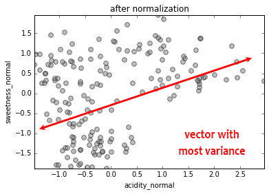
Standardization
To make features comparable, they must be normalized so that
mean = 0 and standard deviation = 1.
(Every data point, subtract mean, divide by std. dev.)
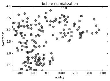
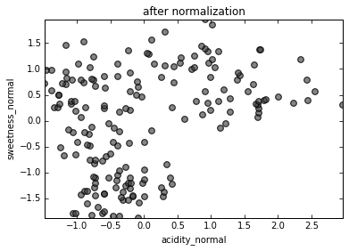
Without normalization, acidity would determine statistics more than sweetness simply because its units are measured in the thousands.
Normalized data is important for some
parametric algorithms
The K-Means algorithm
K-Means is the "go-to" algorithm for unsupervised machine learning, generally what everyone uses unless there's a reason to use something different.
It is robust and flexible and it scales well: if you have a lot of instances, random subsampling usually gives comparable results.
Its main drawback is you need to know how many clusters there are beforehand.
The K-Means algorithm
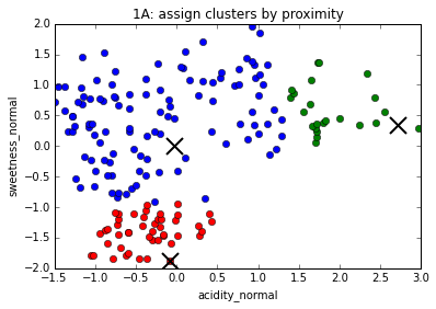
1. Choose number of clusters, k (in this case, 3)
The K-Means algorithm
1. Choose number of clusters, k (in this case, 3)
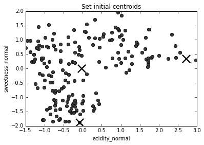
2. Assign (usually randomly) starting position for centroid of each cluster
The K-Means algorithm
1. Choose number of clusters, k (in this case, 3)
2. Assign (usually randomly) starting position for centroid of each cluster
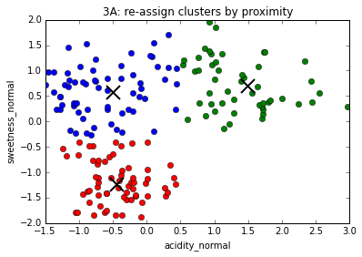
3. Assign every data point to a cluster based on proximity to centroid
The K-Means algorithm
1. Choose number of clusters, k (in this case, 3)
2. Assign (usually randomly) starting position for centroid of each cluster
3. Assign every data point to a cluster based on proximity to centroid
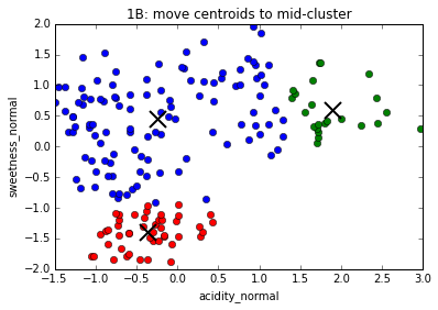
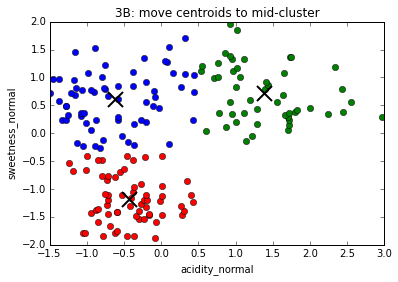
4. Move centroids to geometrical center of points assigned to them
The K-Means algorithm
1. Choose number of clusters, k (in this case, 3)
2. Assign (usually randomly) starting position for centroid of each cluster
3. Assign every data point to a cluster based on proximity to centroid
4. Move centroids to geometrical center of points assigned to them
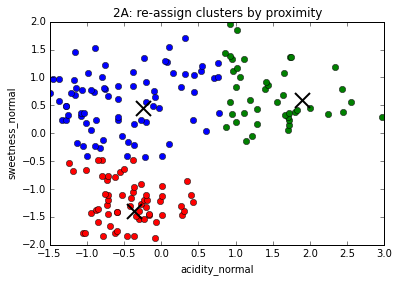
5. Repeat #3
The K-Means algorithm
1. Choose number of clusters, k (in this case, 3)
2. Assign (usually randomly) starting position for centroid of each cluster
3. Assign every data point to a cluster based on proximity to centroid
4. Move centroids to geometrical center of points assigned to them
5. Repeat #3
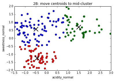
6. Repeat #4
The K-Means algorithm
1. Choose number of clusters, k (in this case, 3)
2. Assign (usually randomly) starting position for centroid of each cluster
3. Assign every data point to a cluster based on proximity to centroid
4. Move centroids to geometrical center of points assigned to them
5. Repeat #3
6. Repeat #4
Keep repeating ...
The K-Means algorithm
1. Choose number of clusters, k (in this case, 3)
2. Assign (usually randomly) starting position for centroid of each cluster
3. Assign every data point to a cluster based on proximity to centroid
4. Move centroids to geometrical center of points assigned to them
5. Repeat #3
6. Repeat #4
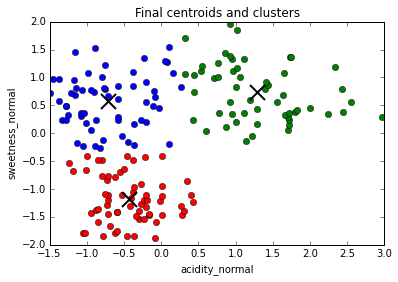
Keep repeating ...
... until convergence, i.e. clusters centers do not move from one repetition to the next
Dependence on initial conditions
The final cluster assignments are dependent on the starting positions of the cluster centers.
When there are very dense clusters separated by very low density regions, cluster centers can get "stuck together"
The solution to both of these problems is to run the algorithm multiple times and assign every point to a cluster based on the frequency
of cluster assignments
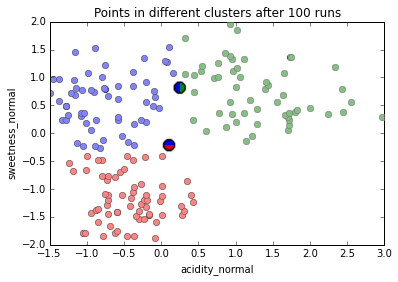
Running K-Means (k=3) on our data 100 times, only two points ever get assigned to different clusters in different runs.
Comparing different values of k
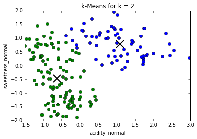
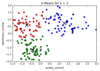
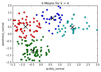
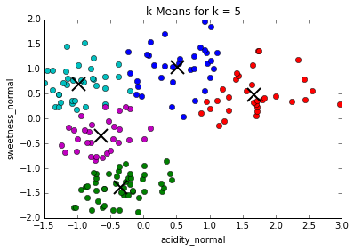
Determining best value for k
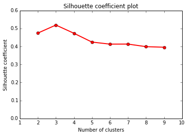
The problem of needing to choose the final number of clusters before running the algorithm can be solved by running it consecutively with increasing number of centers and maximizing the "silhouette coefficient": a (somewhat involved) comparison between intra-cluster distances and the lowest inter-cluster distance for each point. (This is much more computationally expensive)
In our case, the silhouette coefficient shows that, indeed, the optimal value for k = 3.
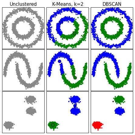
Some other clustering algorithms
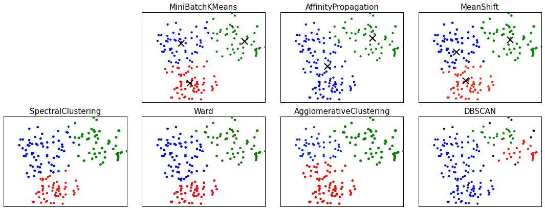
Different algorithms may give different clusters, especially if the clusters are non-globular.
Here are some different algorithms on the fruit data.
Some other clustering algorithms
1) Centroid-based, like K-Means
Some other clustering algorithms
1) Centroid-based, like K-Means
2) Hierarchical, which starts by assembling the closest or separating the furthest points
Some other clustering algorithms
1) Centroid-based, like K-Means
2) Hierarchical, which starts by assembling the closest or separating the furthest points
3) Neighborhood growers, which finds high-density areas and grows them outwards
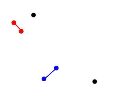
2) Hierarchical Clustering
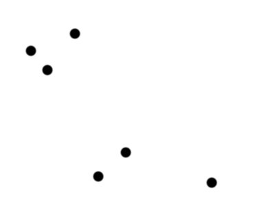
This example is a lot simpler than commonly used hierarchical clustering algorithms like Ward clustering; it's presented with a toy dataset with six points.
We therefore currently have six clusters, each of one point.
An example of bottom-up hierarchical clustering
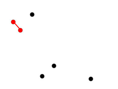
Make a cluster with the two points that are closest together.
Five clusters of size [2, 1, 1, 1, 1]
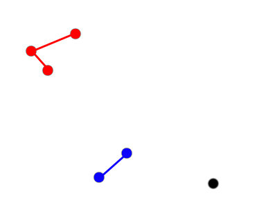
2) Hierarchical Clustering
An example of bottom-up hierarchical clustering
Make a cluster with the next two closest clusters.
Four clusters: [2, 2, 1, 1]
2) Hierarchical Clustering
An example of bottom-up hierarchical clustering
The next two closest points add to the first cluster.
Three clusters: [3, 2, 1]
Like K-Means, we need to decide how many clusters to end up with. Do we stop here, or continue one more step to have two clusters, one red, one blue?
(Can use shadow coefficient again)
If we had done a naive top-down heirarchical clustering , starting with one six-point cluster and dividing twice based on longest distances, we would arrive at the same result.
2) Hierarchical Clustering
An example of bottom-up hierarchical clustering
DBSCAN
3) Neighborhood Grower example:
Neighborhood growers consider local rather than global distances, so are much better at non-globular clusters.
One of the most successful neighborhood growing algorithms is DBSCAN,
"Density-Based Spatial Clustering of Applications with Noise."
DBSCAN
Unlike K-Means and hierarchical clustering, we do not have to choose the number of clusters first; instead this is determined for us based on the densest regions.
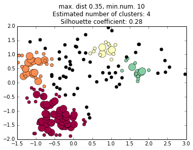
Large circles are "core points"
Small circles are "density-reachable"
points in the same cluster
Black circles are "noise points"
not assigned to a cluster; they could be assigned later with KMeans, starting in the DBSCAN-identified cluster centers.
3) Neighborhood Grower example:
DBSCAN
We do not choose the number of clusters a priori, but we do have to choose the criteria the algorithm uses to decides what regions are dense enough to be considered a cluster core.
We must choose two parameters: the minimum number of points in a cluster core, and the maximum distance between any two points in a cluster core.
These can be thought of as vaguely analogous to mass and volume terms in density in the physical world.
The values of these terms profoundly affects the final cluster determinations, and choosing them can be an art in itself.
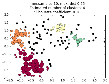
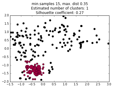
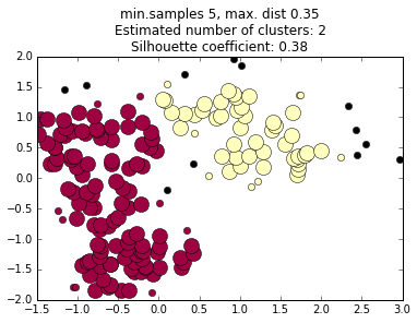

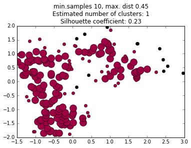
increasing minimum distance
decreasing minimum samples
We're done clustering;
Let's do some
Supervised
Machine Learning
of our fruit dataset
... right after we find out what that means!
Unsupervised
Data starts without labels, everything is measured
Trying to find patterns that then become labels
e.g. here are a bunch of fruit, are there groups ("clusters") of fruit that are more similar to each other than they are to the rest?
If so, maybe -- maybe -- they are different kinds of fruit.
EXPLORATORY Data Analysis
Supervised
Data starts with labels AND measurements ("features")
Trying to find patterns in the measurement that are associated with labels, so that if there are new instances and features, we can predict the new label.
(e.g. a new fruit of a certain color, elongatedness, weight, acidity and sweetness -- what kind of fruit is it?)
PREDICTIVE data analysis
Our fruit dataset

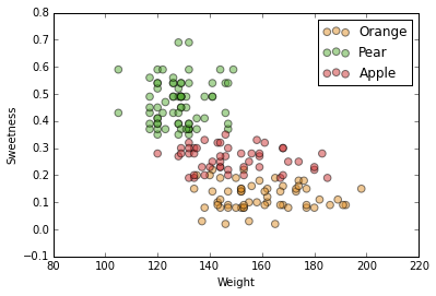
Our fruit dataset + labels
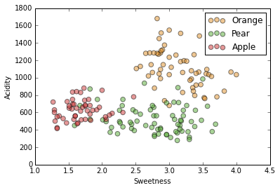
We have three fruits: orange, apple and pear.
We know their acidity, sweetness, weight, elongatedness and color.
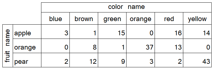
Remember, some of our feature assignment was done by colorblind people, adding "noise".
A label is just a column, or feature,
or variable like all the others.
The only difference is the variable is unknown for new instances; it must be predicted
If the label is a category (e.g. fruit, or even color), we call Supervised Learning "classification".
If it is continuous and numeric (e.g. if we wanted to predict how sweet a new fruit will be), we call it "regression".
Unsupervised:
Data → "Labels" (clusters)
Supervised:
Data + Labels + New Data → New Labels
Again, we'll use two dimensions of our dataset for ease of visualization.
Same two dimensions, acidity and sweetness, but with axes flipped so we "forget" our clusters.
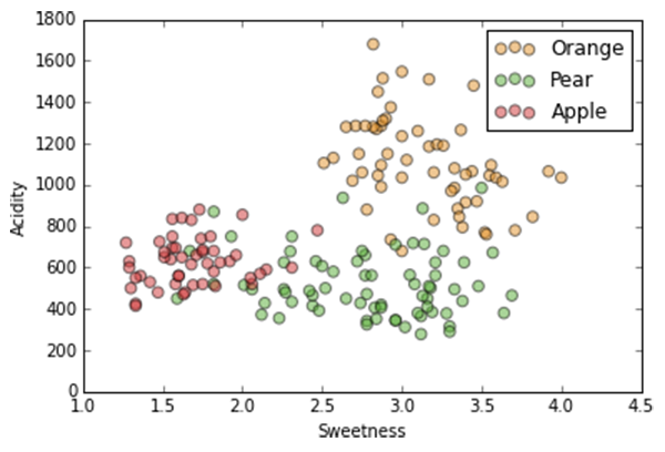
We have this data with these labels...
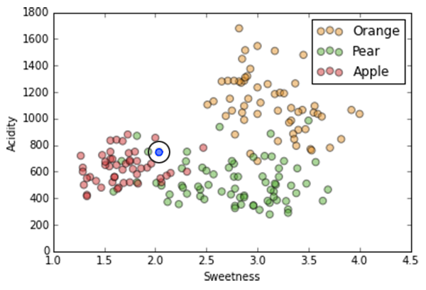
Again, we'll use two dimensions of our dataset for ease of visualization.
Same two dimensions, acidity and sweetness, but with axes flipped so we "forget" our clusters.

If we have a new data point (in blue), what label should we assign it?
There are many classification algorithms; often it doesn't matter which one you use. Except when it does matter.
We'll look at two for pedagogical purposes:
K-Nearest Neighbor and Decision Tree.
K-Nearest Neighbor
It's pretty simple conceptually.
For each new point, choose the label that the majority of k neighbors have.
Note: the "k" in k-nearest neighbor stands for something different than the "k" in k-means; they're both an integer parameter of the algorithm, however.

K-Nearest Neighbor
It's pretty simple conceptually.
For each new point, choose the label that the majority of k neighbors have.
If k=1,
the label is determined by the single closest neighbor, in this case a pear (green)
K-Nearest Neighbor
It's pretty simple conceptually.
For each new point, choose the label that the majority of k neighbors have.
If k=3,
the nearest neighbors are two apples and one pear, so majority vote makes this point an apple.
(It's usually a good idea for k to be an odd number to minimize ties)
K-Nearest Neighbor
It's pretty simple conceptually.
For each new point, choose the label that the majority of k neighbors have.
We now have the exact same problem we had with K-Means:
What's the best value of k?
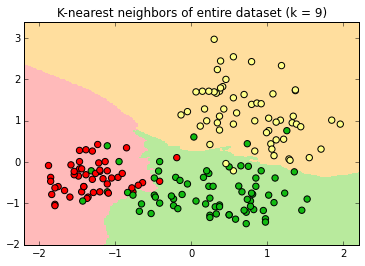
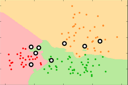
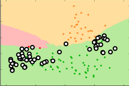
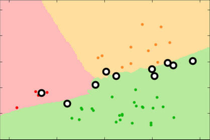
The classifier produces "decision surfaces" that determine the label of new data. Any new point in, e.g. the red region, would be classified an apple.
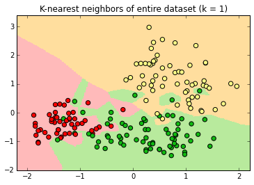
If k=1, the single closest point determines the new label.
Every point has a "halo" around it.
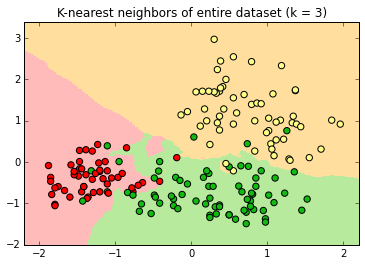
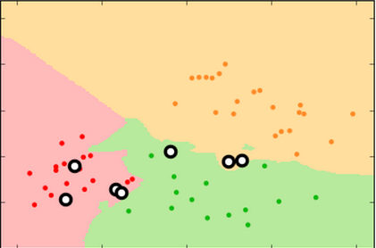
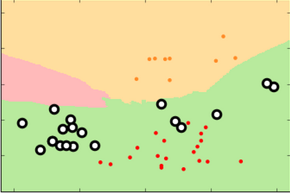
If k=3, the new label is determined by a two-out-of-three "majority vote" of nearest neighbors.
The decision surface is simpler; some points do not have "halos" around them
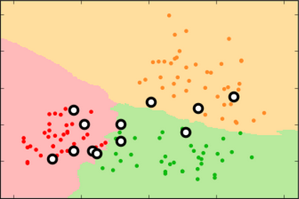
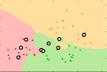
At k=9 there are no halos, just three decision surfaces with sometimes jagged borders.
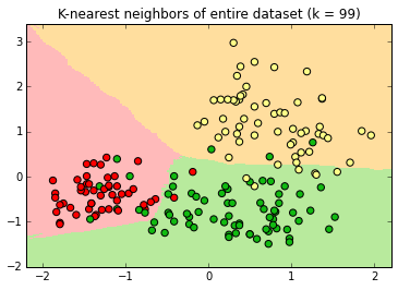
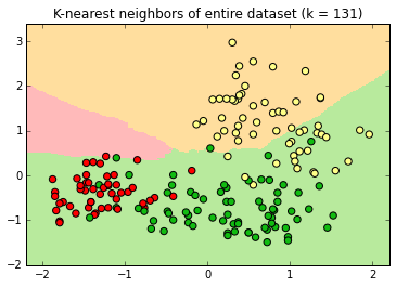
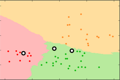
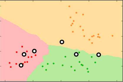
At k=99 , the decision surface edges are relatively smooth. Note the extension of the green surface in the lower left.
At k=131 , the apple decision surface has shrunk considerably into a space with no instances.

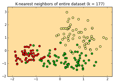
At its maximum value, k=177 , every new label is "orange" because there are more orange instances than apple or pear instance in the dataset.
How do we choose our value of k?
This is called "fitting" the algorithm.
Think of a classifier as a function approximation. There is a "true" function that produced the labels, that we will never know but we try to approximate with a model.
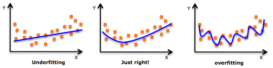
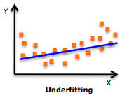
We can visualize this with a simple model, a best-fit regression of a curved dataset made of signal and noise.
If our model is too simple, we are "underfitting", i.e. the model does not adequately represent the signal.
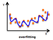
If our model is too complex, we are "overfitting", i.e. we are fitting noise instead of signal.
We try to fit as much signal as possible, without noise.

Large k is underfitting. Our model is too simple as does not take into account all of our data. New data in the region of apple instances will be misclassified as pears.
Small k is overfitting. Our model is too complex. New data in the region of apple instances might be misclassified as pears in certain areas.
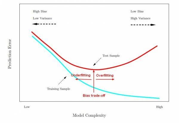
Machine Learning uses special terminology:
"the bias-variance tradeoff"
underfitting = bias
i.e. the model is biased and does not reflect all the signal
overfitting = variance
i.e. the model reflects the noise, or variance, not the signal.
How do we choose the right model to
balance bias and variance?
(in k-nearest neighbor, how do we choose the right k?)
By randomly sequestering part of our data as a testing set; the remaining data becomes our training set.
data
training
70%
testing
30%
Always keep your training and testing data separate.
If you "cheat", you're only cheating yourself
out of a valid model.
A common approach is to randomly split the data into, e.g. five 20% test sets, and build five models, each time using the remaining 80% as a training set.
This is called five-fold cross-validation.
What does testing data sequestration tell you?
When the error rate in the test sample is at a minimum, we are fitting our model well.
kNN is a good algorithm to show bias-variance because the value of k profoundly affects the model's complexity
high k low k
Proper fitting not only minimizes the error rate, it produces more reproducible decision surfaces/models (compare the shapes of the green areas in each replicate for the three conditions)
k=99 k=15 k=3
training set
test set
Proper fitting not only minimizes the error rate, it produces more reproducible decision surfaces/models (compare the shapes of the green areas in each replicate for the three conditions)
k=99 k=15 k=3
test set
new
test
set
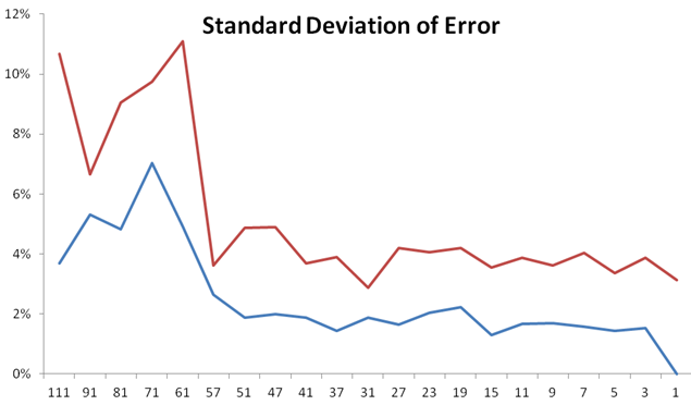
Here is an error rate plot (a.k.a. "learning curve") of our fruit data.
There is quite a wide range of k that fits well.
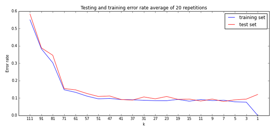
Choosing the right k becomes an optimization scenario. Try a few k's, and find the minimum training set error. (Which may require many repetitions to because of "noise in the error")
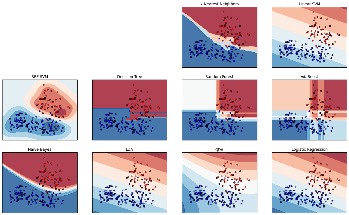
Comparison of classifier algorithms
For simplicity's sake, I collapsed the dataset into two labels, "citrus" (orange, in red) and "non-citrus" (pear and apple, in blue)
Here is our familiar k-Nearest Neighbor classifier.
Different classifiers have differently shaped
decision surfaces...
Linear,
Linear,
Smoothly curved,
Linear,
Smoothly curved,
Globular,
Linear,
Smoothly curved,
Globular,
Irregularly curved,
Linear,
Smoothly curved,
Globular,
Irregularly curved,
Some produce more gradient levels of confidence in the classification (lighter shades)
We'll look at these two in more detail soon;
We'll look at these two in more detail soon;
These three are among the most-used, especially by beginners.
It's easy to fit k-Nearest Neighbors, but it's a relatively slow algorithm that slows down a lot when data sets get large, because every point's distance from every other point must be calculated. So how can we fit an algorithm for which we can't simply choose a value of k?
It's easy to fit k-Nearest Neighbors, but it's a relatively slow algorithm that slows down a lot when data sets get large, because every point's distance from every other point must be calculated. So how can we fit an algorithm for which we can't simply choose a value of k?
If we are underfitting, we can:
-
adjust parameters (not as effective in most algorithms as in k-Nearest Neighbors)
-
change to low-bias model, e.g. logistic regression
-
somehow get more features, e.g. measure the starch content of our fruit
-
use an ensemble of high-bias algorithms (more on this later)
It's easy to fit k-Nearest Neighbors, but it's a relatively slow algorithm that slows down a lot when data sets get large, because every point's distance from every other point must be calculated. So how can we fit an algorithm for which we can't simply choose a value of k?
If we are overfitting, we can:
-
adjust parameters (not as effective in most algorithms as in k-Nearest Neighbors)
-
change to high-bias model, e.g. naive bayes
-
use fewer features or do dimensionality reduction on current features (more later)
-
use an ensemble of low-bias algorithms (more on this later)
-
somehow get more data (e.g. measure more fruit)
We've done k-Nearest Neighbors;
now let's try a different supervised learning algorithm.
Decision trees
Basically like a game of "Twenty Questions" with our data.
The algorithm tries to come up with good questions.
If I asked you to play twenty questions, thinking of a famous person, what would be a better first question:
* Is the person male or female?
* Is the person Miley Cyrus?
More information is gained from the first question because no matter the answer, it eliminates a lot of choices.
REPLICATE 1:
Decision tree built on a randomly chosen 70% training set
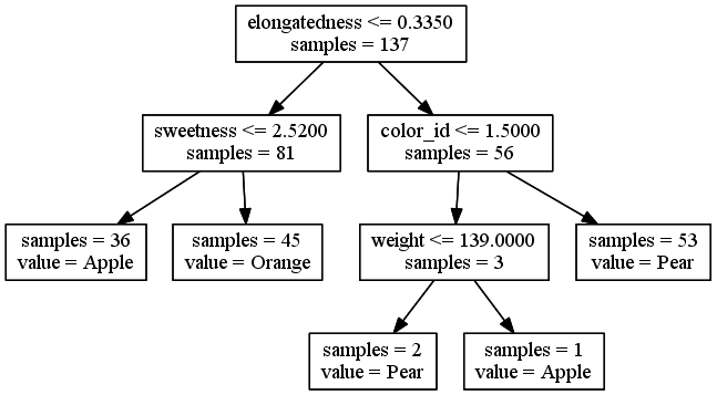
Note: Not all features used (acidity missing)
The last branch is only splitting 3 of 179 instances. Is it overfitting?
This time, only two features were used; this probably means the 70% randomly chosen for the training set did not have enough variation in the other features to justify a split.
We got different models with different training sets. That tells us the fit is probably off, but it doesn't tell us if either of our models is better than the other, i.e. if the more complex one is overfitting or the simpler one is underfitting.
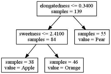
REPLICATE 2:
Decision tree built on another randomly chosen 70% training set
Ensemble methods
In practice, Decision Trees tend to overfit. A lot.
You can adjust the fit by tuning the parameters (e.g. minimum number of instances to split), but there's a better way.
Ensemble methods in machine learning allow you to take overfitting algorithms, run many of them with random parameters in parallel, and "average" them into a model that fits well.
They can also be done with underfitting algorithms.
Random Forest
An ensemble of decision trees
Randomly create tens or hundreds or even thousands of decision trees based on training and test sets, keep the features of the ones that end up with the highest test set accuracy, and build a hybrid tree at the end.
This works surprisingly well, and it tells us the relative importance of different features.
It's a black box, but it's a robust black box.
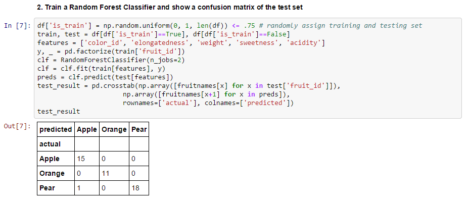
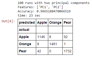
Random Forest
only a few lines of code:
"Confusion Matrix" shows only one error in the test set, a pear misclassified as an apple.
Random Forest
I recommend the Random Forest Classifier to someone just starting out in machine learning.
It uses "bootstrapping" to simulate its own training and test sets, so it in many ways tunes itself.
Once you're comfortable with it, you can start learning other algorithms that give you more ability to fine-tune.
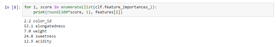
Random Forest
Random Forest Classifiers also give you some interesting info, the relative feature importances:
Elongatedness and sweetness contribute most to the best decision trees;
Color ID and acidity the least.
Random Forest
Let's see what happens when we use all the features to when we used the best two and the worst two only.
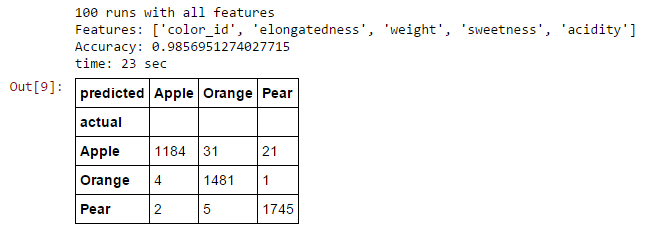
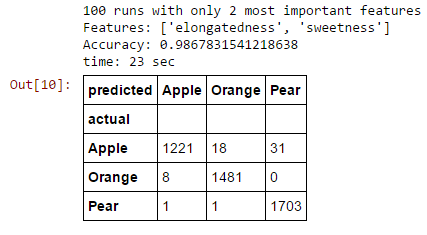

Random Forest
Let's see what happens when we use all the features to when we used the best two and the worst two only.
Fewer features result in slightly higher accuracy. Why? because of...
The Curse of Dimensionality
As you add features, the risk of overfitting increases, and the number of instances you need to fit correctly increases exponentially to the number of features.
Therefore, there is always an optimal number of features.
If you have too many features, you can throw some away, or you can do "dimensionality reduction".
Dimensionality Reduction
A common approach is PCA (Principal Component Analysis). It reduces our number of features while retaining as much information as possible, making "hybrid features" that are combinations of the existing features.
Don't worry if you don't get this part at first,
it takes practice for it to sink in.
PCA
We reduce our five dimensions to two, by identifying each feature's vector of greatest variance compared to every other, and projecting these vectors into two directions in a way that conserves the most overall variance. (Again, don't worry if this is opaque)
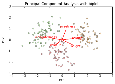
PCA
Our five dimensions have been projected onto two.
The superimposed "biplot" arrow shows the direction and length of each of the original features' vector of maximum variance when projected onto the two new features
'color_id' and 'sweetness' are inversely correlated (except remember that 'color_ID' has an arbitrary number). 'weight' and 'sweetness' are uncorrelated, and 'acidity' and 'weight' are correlated. There is much mutual information that can be compressed to 2 dimensions.
PCA
Our two principal components lose a little accuracy, but it is still quite high.
When you have 1,000 or 1,000,000 features, the difference is much more remarkable.
1,000,000 features?!?!
This can happen very easily in "sparse matrices", which occur often in consumer or language analysis, two important fields in machine learning.
For example, if we tried to classify the following sentences as positive or negative sentiment:
Negative: "I really hate this product."
Negative: "This thing sucks!"
Positive: "This product is so awesome!"
Positive: "I'm happy with my purchase."
Sparse matrices
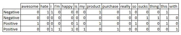
This is called a "bag of words".
15 features > 4 instances
Most values are zero.
You need a non-Euclidean distance function and a high bias algorithm like Naive Bayes because it's very easy to overfit. (What if "awesome" was used ironically?)
Latent features
Another way to think of dimensionality reduction is the discovery of fundamental (latent) properties behind the features you can actually measure.
For example, if your PCA collapses sex, age, height and weight together, the resulting feature might be related to body fat percentage, which was not directly measured.
If a bag of words has a feature composed of "great", "fantastic", "wonderful", "awesome", "cool", the latent feature could be positive sentiment,
In practice, the nature of latent features tends to be a lot more difficult to guess, but if they improve performance, who cares?
Logistic Regression
Another very popular classifier that, confusingly, does classification as well as regression.
We won't go into it here, but among its most popular features is the fact that when you add new training data, you don't have to recalculate the entire classifier from scratch, you can just increment it.
Cost Function
We've been judging our classifiers based on unweighted accuracy, i.e. every correct classification is equally good, every incorrect one is equally bad.
We can weight them, however -- e.g. maybe it's really important that we classify oranges correctly, and maybe we really have to avoid misclassifying apples as pears (but not necessarily vice-versa).
We can optimize our classifier based on any "cost function"
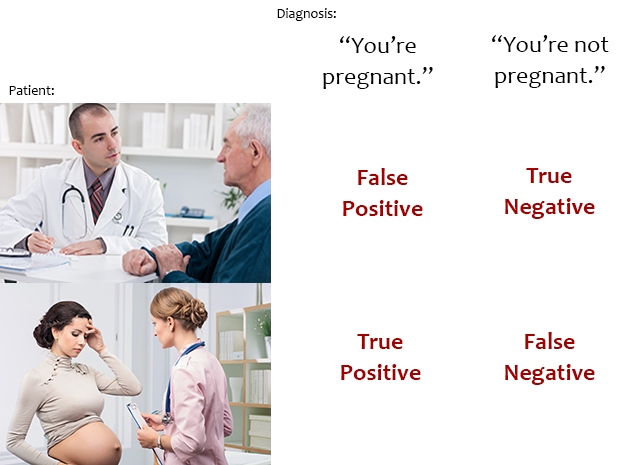
In what kind of classifier would it be more important to minimize false positives or false negatives?
- An adult-content filter for school computers
- A book recommendation classifier for Amazon
- A genetic risk classifier for cancer
Precision & recall
I won't get into these terms, other than to point out they're related to the false positive and negative rates, and they continue machine learning's fine tradition of taking common English words and making them mean something different (although not totally different, which IMO is even worse. I wouldn't get confused if they called the false positive rate the "Batman coefficient" or something).

Intro to data analysis using machine learning (standalone version)
By David Taylor


