REGRESSIONS
Linear Models

Quentin Fayet
About this presentation
This presentation aims to achieve several goals
- Give an insight of the most basic regression model
- Broach the overall philosophy of mathematics models (from mathematics development to code)
- Show that a single problem can be addressed in multiple different ways
About this presentation
However, (linear) regression is a vaste subject, so this presentation won't introduce:
- Data preparation: feature normalization / feature scaling
- Separation between training/testing dataset
- Model validation metrics
What does Regression stands for ?
Regression attempts to analyze the links between two or more variables.
Problem
General problem :
- We have a dataset of :
- Gas consumption over a year in 48 states (US) in M of gallons
- Percent of driving licences
- Assuming that the gas consumption is a linear function of the percent of driving licences
As we have a single feature, this is Simple Linear Regression
(dataset from http://people.sc.fsu.edu/)
Inputs / Ouputs
Inputs :
- Percent of driving licences (feature n°1)
Outputs:
- Gas consumption
Supervised learning
Loading and Plotting
Part. 1
Raw dataset
9.00,3571,1976,0.5250,541
9.00,4092,1250,0.5720,524
9.00,3865,1586,0.5800,561
7.50,4870,2351,0.5290,414
8.00,4399,431,0.5440,410
10.00,5342,1333,0.5710,457
8.00,5319,11868,0.4510,344
8.00,5126,2138,0.5530,467
8.00,4447,8577,0.5290,464
7.00,4512,8507,0.5520,498
...
Structure : gas tax, avg income, paved highways, % driver licence, consumption
Loading dataset with Pandas
import pandas as pd

petrol = pd.read_csv('petrol.csv',
    header=None,
    names=['tax', 'avg income', 'paved highways', '% drive licence', 'consumption']);
Dataviz
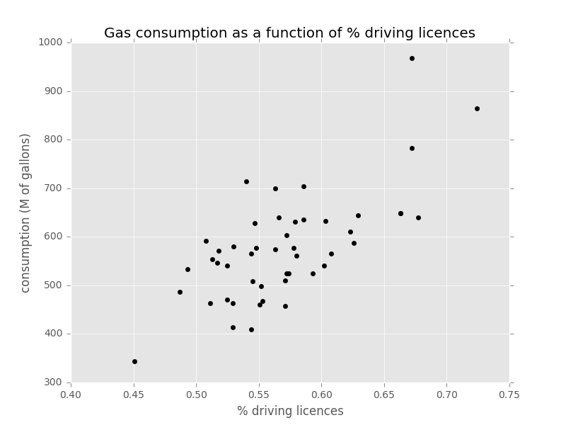
2 dimensions :
import matplotlib.pyplot as plt

def plot():
    plt.scatter(petrol['% drive licence'], petrol['consumption'],  color='black')
    plt.xlabel('% driving licences')
    plt.ylabel('consumption (M of gallons)')
    plt.title('Gas consumption as a function of % driving licences')
    plt.show()
Dataviz
Theory behind Regression
Part. 2 (linear model)
Theory of regression
- One of the most ancient model
- Regressing a set of data to an equation that fits best the data
- Determine the parameters of the equation
Linear Regression : Scalar
For a set of features variables and 1 output variable :
n
y^* = h_\theta(x_1, \cdots, x_n) = \theta_0 + \theta_1 x_1 + \cdots + \theta_n x_n
: explained variable (the predicted output)
: hypothesis parameterized by Theta
: parameters (what seek to determine)
: explainatory variables (the given inputs)
y^*
h_\theta
\theta_0, \cdots, \theta_n
x_1, \cdots, x_n
Linear Regression : Our case
y^*_{consumption} = \theta_0 + \theta_1 \times x_{pct\_driving\_licences}
We have :
- 1 feature (explainatory variable) :
- Percent of driving licences
- An output (explained variable) :
- Gas consumption
Finding would perform the regression
\theta_0, \theta_1
Linear Regression : Vector
When the number of features grows up, scalar notation is inefficient
n
y^* = h_{\hat{\theta}}(\hat{x}) = \hat{\theta}^T \hat{x}
: explained variable (the predicted output)
: hypothesis parameterized by vector Theta
: vector of parameters (what seek to determine)
: vector of explainatory variables (the given inputs)
y^*
h_{\hat{\theta}}
\hat{\theta} \in \space \mathbb{R}^{n+1}
\hat{x} \in \space \mathbb{R}^{n+1}
: Transpose vector of parameters
\hat{\theta}^T
Linear Regression : Our case
Considering a single input :
- Percent of driving licences
\hat{x} = \begin{pmatrix} 1 \\ x_{pct\_driving\_licences} \end{pmatrix} \in \space \mathbb{R}^2
\hat{\theta} = \begin{pmatrix} \theta_0 \\ \theta_1 \end{pmatrix} \in \space \mathbb{R}^2
Linear Regression : Matrix
Represents prediction over the whole dataset and features in a single equation. For inputs of features:
\hat{y}^* = h_{\hat{\theta}}(X) = X^T \hat{\theta}
: vector or explained variable (the predicted outputs)
: hypothesis parameterized by vector Theta
: vector of parameters (what seek to determine)
: matrice of explainatory variables
\hat{y}^* \in \space \mathbb{R}^m
h_{\hat{\theta}}
\hat{\theta} \in \space \mathbb{R}^{n+1}
X \in \space \mathbb{R}^{m \times n+1}
: Transpose matrice of explainatory variables
X^T
m
n
Hypothesis implementation
Using numpy, we can easily implement the hypothesis as a matrice product:
import numpy as np

def hypothesis(X, theta):
    return np.dot(X, theta)
Linear Regression : Our case
If we'd like to batch predict 30 gas consumptions :
X = \begin{pmatrix} \hat{x}_1^T \\ \vdots \\ \hat{x}_{30}^T \end{pmatrix} \in \space \mathbb{R}^{30 \times 2} = \begin{pmatrix} \begin{pmatrix} 1 & x_{1,pct\_driving\_licences} \end{pmatrix} \\ \vdots \\ \begin{pmatrix} 1 & x_{30,pct\_driving\_licences} \end{pmatrix} \end{pmatrix}
\hat{\theta} = \begin{pmatrix} \theta_0 \\ \theta_1 \end{pmatrix} \in \space \mathbb{R}^2
\hat{y}^* = \begin{pmatrix} y_1^* \\ \vdots \\ y_{30}^* \end{pmatrix} \in \space \mathbb{R}^{30}
Training a common linear model : LMS
Part. 3
Least Squares
Goal is to minimize the sum of the squared errors
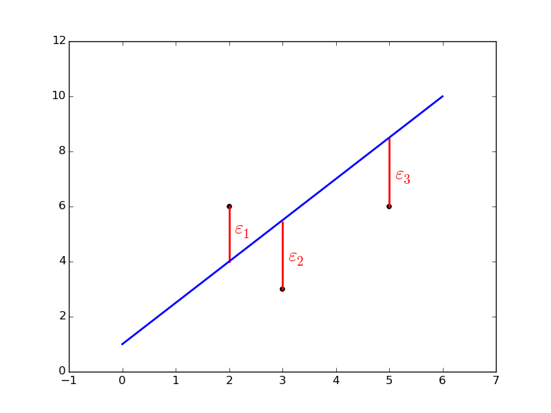
sumOfErrors = \left|\varepsilon_1\right| + \left|\varepsilon_2\right| + \left|\varepsilon_3\right|
Least Squares
is actually the difference between the prediction and the actual value :
\varepsilon
\varepsilon = \left|y^* - y\right|
Thus, the prediction is the result of the hypothesis :
\varepsilon = \left|h_{\hat\theta}(\hat{x}) - y\right|
Least Squares
Generalizing for entries, total error is given by:
m
\varepsilon = \sum\limits_{i=1}^m \left|h_{\hat\theta}(\hat{x}_i) - y_i\right|
Thus, total squared error is (the cost function):
J(\hat{\theta}) = \sum\limits_{i=1}^m (h_{\hat\theta}(\hat{x}_i) - y_i)^2
Least Squares
Lets implement the error (piece of cake thanks to numpy arrays):
import numpy as np

def error(actual, expected):
    return actual - expected
And the squared errors:
import numpy as np

def squared_error(actual, expected):
    return error(actual, expected) ** 2
Least Squares
Finally, we need to minimize the sum of least squares:
\min\limits_\theta \sum\limits_{i=1}^m (h_{\hat\theta}(\hat{x}_i) - y_i)^2
This is called Ordinary Least Squares
Least Squares
We may sometimes encounter an other notation:
\min\limits_\theta \left||h_{\hat{\theta}}(\hat{x}_i) - y_i\right||^2_2
Which is the same, using l2-norm regularization notation
\min\limits_\theta \left||h_{\hat{\theta}}(\hat{x}_i) - y_i\right||^2
Least Squares
Plotting the cost function gives an insight on the minimization problem to be solved:
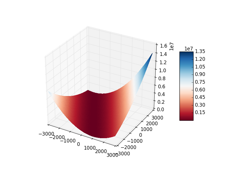
Least Squares
For Mean Least Squares we take the average error over the dataset
\min\limits_\theta \frac{1}{2m} \sum\limits_{i=1}^m (h_{\hat\theta}(\hat{x}_i) - y_i)^2
Hence, for inputs, we have:
m
stands to make derivate simplier.
\frac{1}{2}
Gradient descent
Gradient descent is one of the possible way to solve the optimization problem.
Repeat until convergence :
\theta := \theta - \alpha \nabla J(\hat{\theta})
{
}
: learning rate
: partial derivative of over
\alpha
\nabla J(\hat{\theta})
J(\hat{\theta})
\theta_j
Gradient descent
Once the partial derivative applied, we obtain:
Repeat until convergence :
\theta_j := \theta_j + \alpha \sum\limits_{i=1}^m(y_i - h_{\hat{\theta}}(\hat{x}_i))x_i^{(j)}
{
}
Gradient descent
Let's implement the batch gradient descent:
import numpy as np
from hypothesis import hypothesis
from squared_error import squared_error, error
def gradient_descent(X, y, theta, alpha, iterations = 10000):
X_transpose = X.transpose()
m = len(X)
for i in range(0, iterations):
hypotheses = hypothesis(X, theta)
cost = np.sum(squared_error(hypotheses, y)) / (2 * m)
gradient = np.dot(X_transpose, error(hypotheses, y)) / m
theta = theta - alpha * gradient
print("Iteration {} / Cost: {:.4f}".format(i, cost))
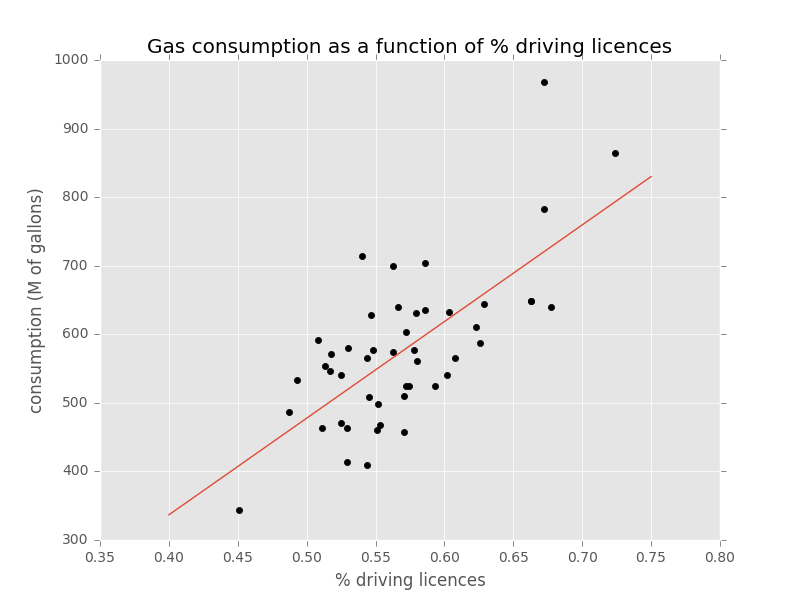
return thetaTraining with Gradient descent
When running the gradient descent on the dataset, we obtain the following parameters:
\theta_0 = -227.07
\theta_1 = 1409.43
Considering the following:
\alpha = 0.05
iterations = 70,000
\hat{\theta} = \begin{pmatrix} 0 \\ 0 \end{pmatrix}
Plotting the linear function
Other ways to solve the optimization problem
Gradient descent (batch / stochastic) are not the only ways.
- Conjugate Gradient Descent: Finite number of iterations
- Normal equation: non iterative way
- BFGS / L-BFGS: Non-linear models. No need to choose the learning rate. Convergence happens faster
A tour of the
linear models using Scikit-learn
Part. 4
Common models
- Least Squares :
- Ordinary Least Squares
- Ridge
- Lasso
- Elastic Net
- Least Angles (High dimensional data)
- LARS Lasso
- OMP
Ordinary Least Squares
Using scikit-learn, performing OLS regression is easy:
from sklearn import linear_model
# Dataset has been previously loaded as shown
# Instanciate the linear regression object
regression = linear_model.LinearRegression()
# Train the model
regression.fit(petrol['% drive licence'].reshape(-1, 1),
pretrol['consumption'])
coeffectients = regression.coef_ #1-D array in Simple Linear Regression
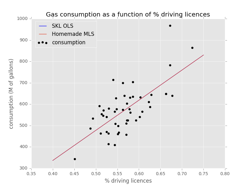
intercept = regression.intercept_Ordinary Least Squares
Training gives us the following coefficients:
print('Intercept term: \n', regr.intercept_)
print('Coefficients: \n', regr.coef_)
\hat{\theta} = \begin{pmatrix} -227.31 \\ 1409.84 \end{pmatrix}
Ordinary Least Squares
Plotting against our own implementation:
Ridge regression
Ridge regression penalizes the collinearity of the explainatory variables by introducing a shrinkage amount
Minimizes the "ridge" effect
Ridge regression
The optimization problem to solve is slightly different:
\min\limits_\theta \sum\limits_{i=1}^m (h_{\hat\theta}(\hat{x}_i) - y_i)^2 + \alpha \sum\limits_{i=0}^{n} \theta_i^2
\min\limits_\theta \left||h_\theta(\hat{x}_i) - y_i\right||^2 + \alpha \left||\theta\right||^2
Using l2-norm regularization on both error and parameters
is the shrinkage amount
\alpha
Ridge regression
Ridge regression makes sense in multivariables regression, not in Simple Linear Regression as it penalizes multicollinearity
from sklearn import linear_model
# Dataset has been previously loaded as shown
# Instanciate the linear regression object
regression = linear_model.Ridge(alpha=.01)
# Train the model
regression.fit(petrol['% drive licence'].reshape(-1, 1),
pretrol['consumption'])
coeffectients = regression.coef_
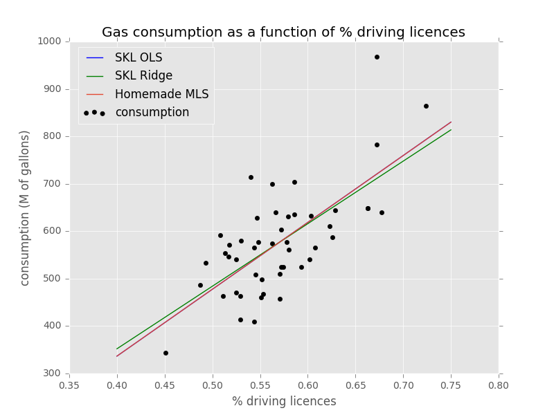
intercept = regression.intercept_Ridge regression
Training gives us the following coefficients:
print('Intercept term: \n', regr.intercept_)
print('Coefficients: \n', regr.coef_)
\hat{\theta} = \begin{pmatrix} -175.30 \\ 1318.66 \end{pmatrix}
Ridge regression
Plotting against other methods:
Lasso Regression
Lasso Regression is particularly efficient on problems where the number of features is much bigger than the number of entries in the training dataset:
It highlights some features and minimizes some others
n >> m
The optimization problem to solve:
Using l2-norm regularization on error and l1-norm on parameters
Lasso Regression
\min\limits_\theta \sum\limits_{i=1}^m (h_{\hat\theta}(\hat{x}_i) - y_i)^2 + \alpha \sum\limits_{i=0}^{n} |\theta_i|
\min\limits_\theta \left||h_\theta(\hat{x}_i) - y_i\right||^2 + \alpha \left||\theta\right||_1
Lasso regression
Ridge regression makes sense in multivariables regression, not in Simple Linear Regression as it penalizes multicollinearity
from sklearn import linear_model

# Dataset has been previously loaded as shown

# Instanciate the linear regression object
regression = linear_model.Lasso(alpha=.1)

# Train the model
regression.fit(petrol['% drive licence'].reshape(-1, 1),
                                pretrol['consumption'])

coeffectients = regression.coef_
intercept = regression.intercept_
Lasso regression
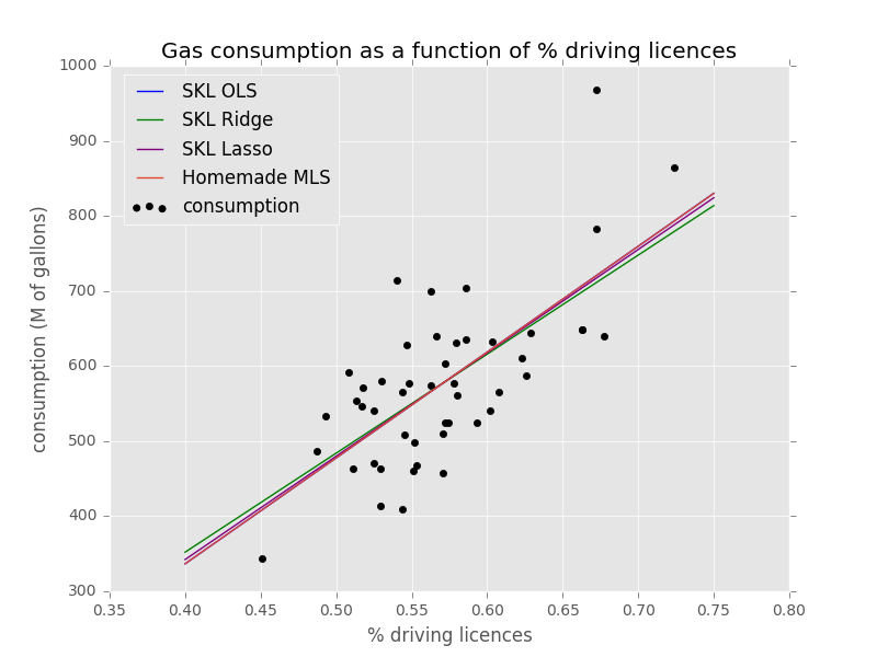
Training gives us the following coefficients:
print('Intercept term: \n', regr.intercept_)
print('Coefficients: \n', regr.coef_)
\hat{\theta} = \begin{pmatrix} -208.38 \\ 1376.65 \end{pmatrix}
Lasso regression
Plotting against other methods:
Conclusion
Part. 5
Conclusion
- Linear Regression is the simpler regression, yet:
- it may addresses a lot of problems (classification, ...)
- it is very vaste
- it is still used as the basis of a great variety of algorithms
ML : Regressions - linear models
By quentinfayet
ML : Regressions - linear models
Slides about linear models for regression in Machine Learning