Introduction To Feature Selection

Learning an Art . Not a Science .

Computer Science Sophomore
Machine Learning Enthusiast
Web Scraping
Python Lover
Researcher

Machine Learning Pipeline

What are Features ?

Also known as Independent Variables or Predictors Help us to PREDICT the Target Variable or Response .
Features help us to describe our problem .They are what help us to determine/predict the Target Variable or Response .
Features may be Continous or Categorical .

Types Of Features

Features

Continous

Categorical

Income
House Prices
Height

Gender
Grade
Colour

Feature Selection

Feature Selection is a very important step while building Machine Learning Models .

Feature Selection is the process of selecting those attributes or features from our given pool of features that are most relevant and best describe the relationship between Predictors and Response .

One important thing to keep in mind is that it is different from Dimensionality Reduction . In Feature Selection , we simply mute / remove the features irrelevant to us without changing them whereas in Dimensionality Reduction (such as PCA) , the number of features are reduced by making combinations of our existing features .

The What ?

Feature Selection

Feature Selection helps to remove the irrelevant data which either does not contribute at all to the accuracy of our predictive model but in some cases may even be dampening it .

Feature Selection is desirable because :

1. It helps to escape the 'Curse Of Dimensionality' .

2. They help to remove the noise caused by the undesirable attributes .

3. They reduce the complexity of the model which makes the intuition behind the results of the model comprehendible .

Example : For Brain Tumour Classification , the number of features available can range from 6000 to 60,000 !!

The Why ?

Curse Of Dimensionality

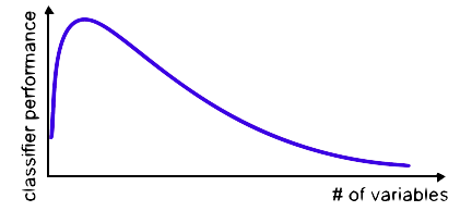
The amount of data required to achieve the same level of accuracy increases exponentially as the number of features increases .

But in practise , the volume of training data available to us is fixed . Therefore , in most cases , the performance of the classifier will decrease with an increased number of variables .

Feature Selection Methods

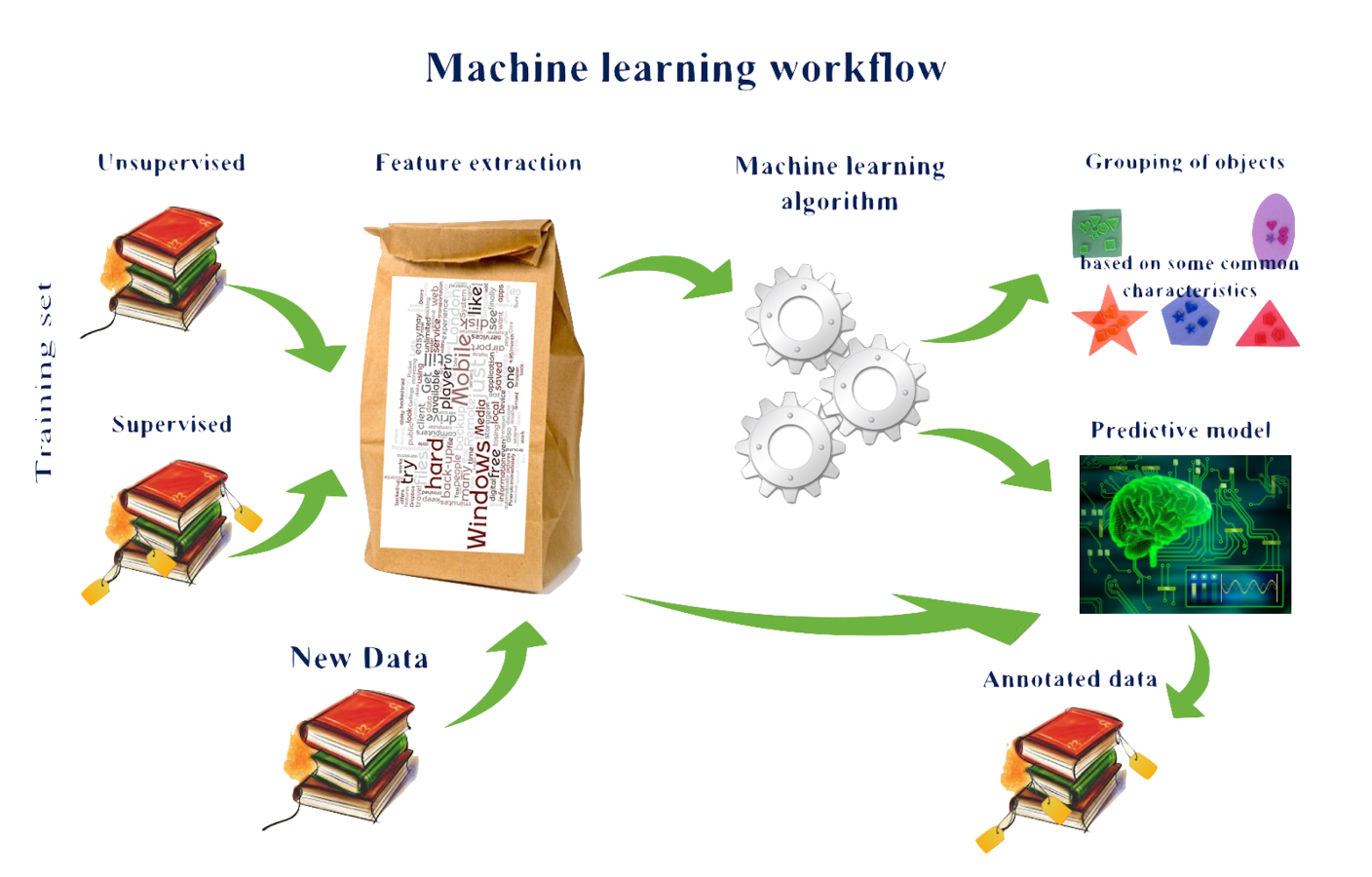
Feature Selection Algorithms can be broadly classified into 3 classes :

Filter Methods
Wrapper Methods
Embedded Methods

Filter Methods

Filter Methods form the First Class of Feature Selection Algorithms .

What we do here is that we apply a statistical test to infer the relationship between the response and predictors .

The tests are mostly bivariate ( applied on two quantities ) and consider the response with one of the features .

What Happens

Filter Methods are purely Statistical in nature and the process of Feature Selection is completely independent of the Machine Learning Algorithm .

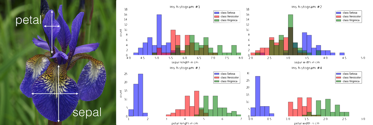
They are mainly used as a Pre-Processing step and are great for visualising the data to infer some intuitive and some not-so intuitive patterns in the data .

	Categorical	Continous
Categorical	Chi-Square	Anova
Continous	LDA	Pearson Correlation

Feature

Response

Pearson's Correlation

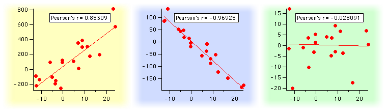
This test is used when both of our Feature and Response are Continous.

The output of Pearson's Correlation is a number (Pearson's Correlation Coefficient) whose value lies in the range of [-1,1] .

Test Inference

A value of -1 indicates that there is a perfectly negative relationship between the two variables i.e. as one increases , the other decreases .

Similarly , a value of +1 indicates a perfectly positive relationship among the variables .

A value of 0 indicates that there is no kind of relationship at all among the variables .

Computing Pearsons Correlation

from scipy.stats import pearsonr

""" Inputs : x and y which are numpy matrices of the feature and response .
    Output : Pearson Correlation value and P-value which shows the 
             probability of an uncorrelated system producing a correlation 
             coefficient of this magnitude .                                       """

Pearson_Correlation = pearsonr(x,y)

\rho(X,Y) = \frac{{\ Cov}(X,Y)}{\sqrt{{\ Var}(X){\ Var}(Y)}}

\rho(X,Y) = \frac{{\ Cov}(X,Y)}{\sqrt{{\ Var}(X){\ Var}(Y)}}

Mathematical Formulae :

Chi-Square Test

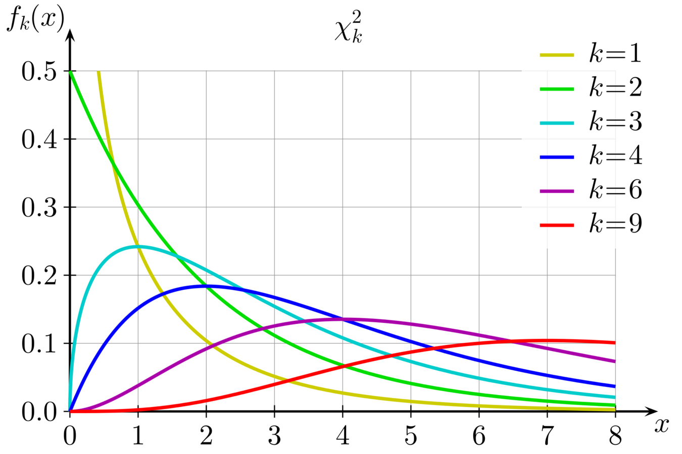
This test is used when our Feature and Response both are categorical .

The Chi-Square Test is a dependency test which helps us to determine wether there is any kind of dependence among the variables under observation or not .

A more statistical way of looking at this test is that it tests the Null Hypothesis that the variables are independent .

Test Inference

For computing the Chi-Square Statistic , two values are computed , namely , Degrees of Freedom and the Chi-Square Value .

Using the above two values , the p-value is computed which has an intuitive significance .

The cutoff value for p-value significance is 0.05 . That is , if the p-value is below that , null hypothesis is rejected which implies that the variables are dependent .

Computing Chi-Square Value

Mathematical Formulae :

\tilde{\chi}^2=\sum_{k=1}^{n} \frac{(O_k - E_k)^2}{E_k}

\tilde{\chi}^2=\sum_{k=1}^{n} \frac{(O_k - E_k)^2}{E_k}

from scipy.stats import chisquare

""" Inputs : x and y which are numpy matrices of the feature and response .
    Output : The chi-square statistic as computed from the above formulae 
             and the p-value .                                            """

Chi_Square = chisquare(x,y)

Wrapper Methods

They form the Second Class of Feature Selection Algorithms .

They work on the basic principles of Combinatorics .

In this method , the learning algorithm (classifier) itself is used to perform the Feature Selection and select the top features .

What Happens ?

The classifier is trained using different combinations (subsets) of features and then the best combination of features is decided upon by looking at the predictive scores .

Therefore , in a way , the problem boils down to a search problem .

The search process maybe methodical such as best-first search or it may stochastic such as random hill climbing problem or it may use heuristics , such as forward and backward propagation (used by Neural Networks ) .

Examples of Wrapper Based Methods are Recursive Feature Elimination and Sequential Forward Selection .

Recursive Feature Elimination

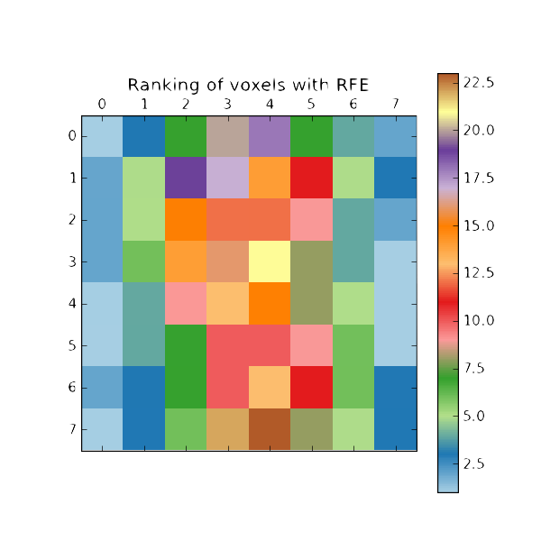
The most common type of algorithm used in Wrapper Based Methods is the Recursive Feature Elimination . It is a Backward Selection Method .

What it does is that it initially takes in all features to build the model and assigns a weight to every feature . It then prunes this feature set recursively by removing the lower weighted features till the desired number of features is reached .

Recursive Feature Elimination is very commonly used with Support Vector Machines (SVM) .

The What ?

Recursive Feature Elimination

from sklearn.feature_selection import RFE
from sklearn.linear_model import LinearRegression

''' Use Linear Regression as the model . '''
Classifier = LinearRegression()
''' Rank all features, i.e. continue the elimination until the last one . '''
Rfe = RFE(Classifier, n_features_to_select=1)
Rfe.fit(X,Y)

print Rfe.ranking

The How ?

Sequential Feature Selection

Another algorithm used in Wrapper Based Methods is the Sequential Feature Selection . It is a Forward Selection Method .

In this method , we start out initially with an empty feature subset and add one feature at a time to this subset till the desired number of features are added to the feature subset .

The What ?

Sequential Feature Selection

The How ?

from mlxtend.feature_selection import SequentialFeatureSelector as SFS
from sklearn.neighbors import KNeighborsClassifier

''' Use KNN Classifier with K =4 '''
Classifier = KNeighborsClassifier(n_neighbors=4)
Sfs = SFS(Classifier,k_features=3, scoring='accuracy')

Sfs.fit(X,y)

print Sfs.subsets_

Embedded Methods

They form the Third Class of Feature Selection Algorithms .

Embedded Methods are dynamic Feature Selection Methods in the sense that they perform the task of Feature Selection while building the model itself .

The features are ranked/selected on the nature of the learning algorithm of the classifier , so the working of the "Black Box" is quite desirable and helpful .

What Happens

In Embedded Methods , what happens is that the process of Feature Selection takes place while the model is being constructed .

So , unlike Wrapper Based Methods , the search for the Feature Set is not accelerated by the accuracy on the validation (held out) set but by the learning process of the classifier used .

Most common examples include : Tree-Based and Regularisation Based Methods .

Regularisation Methods

Regularisation is a way of preventing overfitting and complexity while building machine learning models by adding constraints or penalisation to the model .

So , instead of just optimising the loss function , we optimise the following function :
L(X,Y)+λN(w)
where L(X,Y) is our original loss function and λN(w) is our regularisation term .

Here , λ is a hyper-parameter (value which is to be set by us) which can determined by cross-validation and N(w) is the type of regularisation which can be either L1 or L2 .

L1 (Lasso) Regularisation

In Lasso Regularisation , we simply add the L1-norm of our Feature/Weight Vector to our optimising function . So our optimising function takes the form :
L(X,Y)+λ∑ni|wi|

from sklearn.linear_model import Lasso

''' The argument alpha is for the hyperparameter lambda '''
Regularizer = Lasso(alpha=0.3)
Regularizer.fit(X,y)

''' This prints the coefficients for the different features '''
print Regularizer.coef_

L2(Ridge) Regularisation

In Ridge Regularisation , we add the L2-norm of our Feature/Weight Vector to our optimising function . So our optimising function takes the form :
L(X,Y)+λ∑ni|w2|

from sklearn.linear_model import Ridge

''' The argument alpha is for the hyperparameter lambda '''
Regularizer = Ridge(alpha=0.3)
Regularizer.fit(X,y)

''' This prints the coefficients for the different features '''
print Regularizer.coef_

Overview of Methods

Filter Methods :

Easily Scalable to High Dimensional Data . Computationally fast and simple to implement . Independent of the Machine Learning Algorithm.
Ignores the interactions among the features themselves .

Wrapper Methods :

Takes into account Feature Dependencies . Very Robust in nature .
Very prone to Overfitting . Computationally intensive .

Embedded Methods:

Computationally less expensive than Wrapper Methods with almost similar results (in most cases) .
Specific to a Learning Machine .

Which To Choose ?

QUESTIONS ?

rahulbaboota

rahulbaboota08

Introduction To Feature Selection

By Rahul Baboota

Introduction To Feature Selection

An Introduction to the different methods of Feature Selection in Python .

1,652

Rahul Baboota

Computer Science Junior

Introduction To Feature Selection

Machine Learning Pipeline

What are Features ?

Types Of Features

Features

Feature Selection

Feature Selection

Curse Of Dimensionality

Feature Selection Methods

Filter Methods

What Happens

Pearson's Correlation

Test Inference

Computing Pearsons Correlation

Chi-Square Test

Test Inference

Computing Chi-Square Value

Wrapper Methods

What Happens ?

Recursive Feature Elimination

Recursive Feature Elimination

Sequential Feature Selection

Sequential Feature Selection

Embedded Methods

What Happens

Regularisation Methods

L1 (Lasso) Regularisation

L2(Ridge) Regularisation

Overview of Methods

Introduction To Feature Selection

More from Rahul Baboota