Deep Learning HMC

Building Topological Samplers for Lattice QCD

Sam Foreman

May, 2021

saforem2/l2hmc-qcd

arXiv:2105.03418

MCMC in Lattice QCD

Generating independent gauge configurations is a MAJOR bottleneck for LatticeQCD.

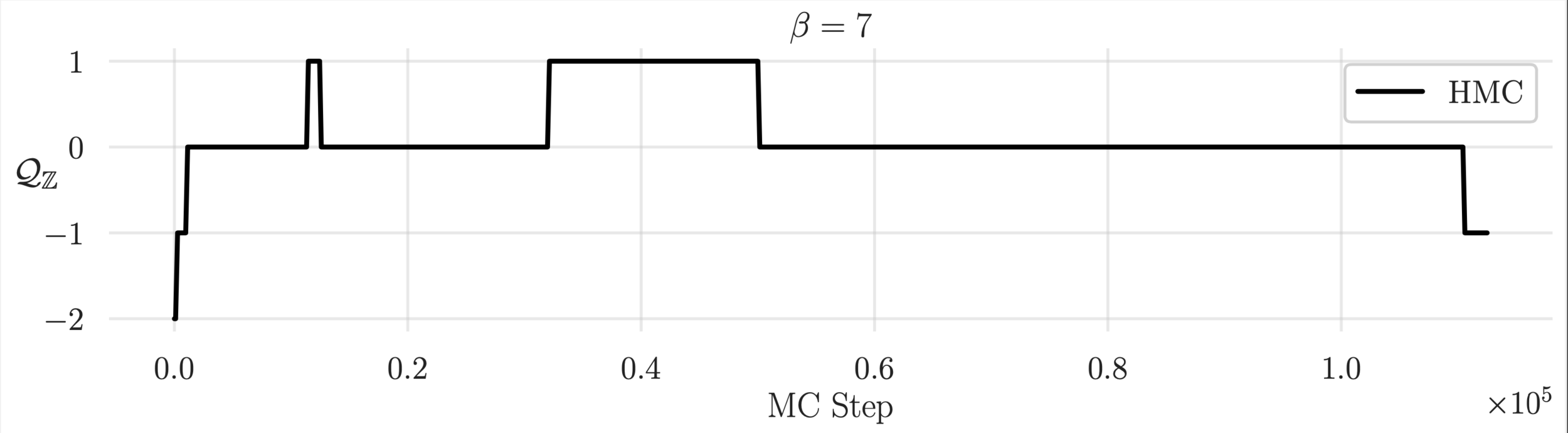
As the lattice spacing, \(a \rightarrow 0\), the MCMC updates tend to get stuck in sectors of fixed gauge topology.
- This causes the number of steps needed to adequately sample different topological sectors to increase exponentially.

Critical slowing down!

Markov Chain Monte Carlo (MCMC)

Goal: Draw independent samples from a target distribution, \(p(x)\)

x^{\prime} = x_{0} + \delta,\quad \delta\sim\mathcal{N}(0, \mathbb{1})

Starting from some initial state \(x_{0}\sim \mathcal{N}(0, \mathbb{1})\) , we generate proposal configurations \(x^{\prime}\)

Use Metropolis-Hastings acceptance criteria

x_{i+1} = \begin{cases} x^{\prime},\quad\text{with probability } A(x^{\prime}|x)\\ x,\quad\text{with probability } 1 - A(x^{\prime}|x) \end{cases}

A(x^{\prime}|x) = \min\left\{1, \frac{p(x^{\prime})}{p(x)}\left|\frac{\partial x^{\prime}}{\partial x^{T}}\right|\right\}

Issues with MCMC

Generate proposal \(x^{\prime}\):

\(x^{\prime} = x + \delta\), where \(\delta \sim \mathcal{N}(0, \mathbb{1})\)

\(\big\{ x_{0}, x_{1}, x_{2}, \ldots, x_{m-1}, x_{m}, x_{m+1}, \ldots, x_{n-2}, x_{n-1}, x_{n} \big\}\)

1. Construct chain:

\(\big\{ x_{0}, x_{1}, x_{2}, \ldots, x_{m-1}, x_{m}, x_{m+1}, \ldots, x_{n-2}, x_{n-1}, x_{n} \big\}\)

2. Thermalize ("burn-in"):

\(\big\{ x_{0}, x_{1}, x_{2}, \ldots, x_{m-1}, x_{m}, x_{m+1}, \ldots, x_{n-2}, x_{n-1}, x_{n} \big\}\)

3. Drop correlated samples ("thinning"):

dropped configurations

Inefficient!

Hamiltonian Monte Carlo (HMC)

Introduce fictitious momentum:

\(v\sim\mathcal{N}(0, 1)\)

Target distribution:

\(p(x)\propto e^{-S(x)}\)

Joint target distribution:

p(x, v) = p(x)\cdot p(v) = e^{-S(x)}\cdot e^{-\frac{1}{2}v^{T}v} = e^{-\mathcal{H(x,v)}}

The joint \((x, v)\) system obeys Hamilton's Equations:

\dot{x} = \frac{\partial\mathcal{H}}{\partial v},

\dot{v} = -\frac{\partial\mathcal{H}}{\partial x}

p(x, v) = p(x|v)p(v)

lift to phase space

v\sim \mathcal{N}(0, \mathbb{1})

\mathcal{H}=\mathrm{const}

HMC: Leapfrog Integrator

(trajectory)

Hamilton's Eqs:

\dot{x}=\frac{\partial\mathcal{H}}{\partial v}, \dot{v}=-\frac{\partial{\mathcal{H}}}{\partial x}

\mathcal{H}(x, v) = S(x) + \frac{1}{2}v^{T}v

Hamiltonian:

(x_{0}, v_{0})\rightarrow \cdots \rightarrow(x_{N_{\mathrm{LF}}}, v_{N_{\mathrm{LF}}})

\(N_{\mathrm{LF}}\) leapfrog steps:

\Longrightarrow

Leapfrog Integrator

x^{\prime} = x + \varepsilon v^{1/2}

v^{\prime} = v^{1/2} - \frac{\varepsilon}{2}\partial_{x}S(x^{\prime})

v^{1/2} = v - \frac{\varepsilon}{2}\partial_{x}S(x)

2. Full-step \(x\)-update:

3. Half-step \(v\)-update:

1. Half-step \(v\)-update:

HMC: Issues

Cannot easily traverse low-density zones.

What do we want in a good sampler?

Fast mixing
Fast burn-in

Mix across energy levels
Mix between modes

Energy levels selected randomly \(\longrightarrow\) slow mixing!

Stuck!

Leapfrog Layer

Introduce a persistent direction \(d \sim \mathcal{U}(+,-)\) (forward/backward)

Introduce a discrete index \(k \in \{1, 2, \ldots, N_{\mathrm{LF}}\}\) to denote the current leapfrog step

Let \(\xi = (x, v, \pm)\) denote a complete state, then the target distribution is given by

p(\xi) = p(x)\cdot p(v)\cdot p(d)

Each leapfrog step transforms \(\xi_{k} = (x_{k}, v_{k}, \pm) \rightarrow (x''_{k}, v''_{k} \pm) = \xi''_{k}\) by passing it through the \(k^{\mathrm{th}}\) leapfrog layer

Leapfrog Layer

where \((s_{v}^{k}, q^{k}_{v}, t^{k}_{v})\), and \((s_{x}^{k}, q^{k}_{x}, t^{k}_{x})\), are parameterized by neural networks

\(x\)-update \((d = +)\):

x^{\prime}_{k} = \Lambda^{+}_{k}(x_{k};\zeta_{x_{k}})

\zeta_{x_{k}}\equiv \big(\quad\odot x_{k}, \partial_{x}S(x_{k})\big)

\bar{m}_{t}

(\(m_{t}\)\(\odot x\)) -independent

\,\quad= x_{k}\odot\exp\left(\varepsilon^{k}_{x}s^{k}_{x}(\zeta_{x_{k}})\right) + \varepsilon^{k}_{x}\left[v^{\prime}_{k}\odot\exp\left(\varepsilon^{k}_{x}q^{k}_{x}(\zeta_{x_{k}})\right)+t^{k}_{x}(\zeta_{x_{k}})\right]

masks:

m_{t}

\bar{m}_{t}

= \mathbb{1}

Momentum (\(v_{k}\)) scaling

Gradient \(\partial_{x}S(x_{k})\) scaling

Translation

\,\quad\equiv\, v_{k}\odot \exp\left(\frac{\varepsilon^{k}_{v}}{2}s^{k}_{v}(\zeta_{v_{k}})\right) - \frac{\varepsilon^{k}_{v}}{2}\left[\partial_{x}S(x_{k})\odot\exp\left(\varepsilon^{k}_{v}q^{k}_{v}(\zeta_{v_{k}})\right) \,+\,t^{k}_{v}(\zeta_{v_{k}})\right]

\zeta_{v_{k}}\equiv \big(x_{k}, \partial_{x}S(x_{k})\big)

\(v\)-update \((d = +)\):

v^{\prime}_{k} = \Gamma^{+}_{k}(v_{k};\zeta_{v_{k}} )

\overbrace{\hspace{80px}}

\overbrace{\hspace{100px}}

\overbrace{\hspace{30px}}

(\(v\)-independent)

Each leapfrog step transforms

\xi_{k} = (x_{k}, v_{k}, \pm)\longrightarrow (x''_{k}, v''_{k}, \pm)=\xi''_{k}

by passing it through the \(k^{\mathrm{th}}\) leapfrog layer.

L2HMC: Generalized Leapfrog

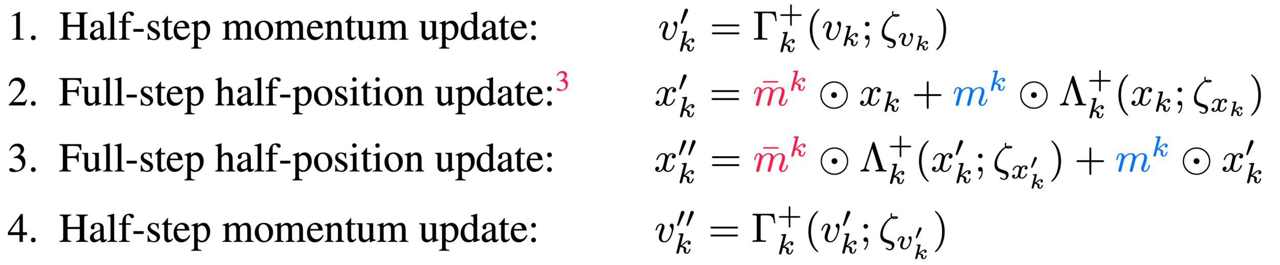
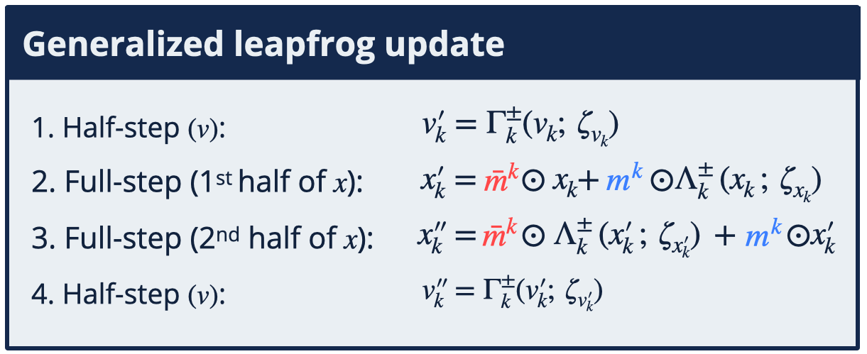
Complete (generalized) update:
1. Half-step \(v\) update:
2. Full-step \(\frac{1}{2} x\) update:
3. Full-step \(\frac{1}{2} x\) update:
4. Half-step \(v\) update:

v^{\prime}_{k} = \Gamma^{\pm}(v_{k};\zeta_{v_{k}})

x^{\prime}_{k} = \hspace{14px}\odot x_{k} + \hspace{14px}\odot \Lambda^{\pm}(x_{k};\zeta_{x_{k}})

\bar{m}^{t}

m^{t}

x^{\prime\prime}_{k} = \hspace{14px}\odot \Lambda^{\pm}_{k}(x^{\prime}_{k};\zeta_{x^{\prime}_{k}}) + \hspace{14px}\odot x^{\prime}_{k}

\bar{m}^{t}

m^{t}

v^{\prime\prime}_{k} = \Gamma^{\pm}(v^{\prime}_{k};\zeta_{v^{\prime}_{k}})

Leapfrog Layer

masks:

Stack of fully-connected layers

Example: GMM \(\in\mathbb{R}^{2}\)

\(A(\xi',\xi)\) = acceptance probability

\(A(\xi'|\xi)\cdot\delta(\xi',\xi)\) = avg. distance

Note:

\(\xi'\) = proposed state

\(\xi\) = initial state

Maximize expected squared jump distance:

\mathcal{L}_{\theta}\left(\theta\right) \equiv \mathbb{E}_{p(\xi)}\left[A(\xi'|\xi)\cdot \delta(\xi',\xi)\right]

Define the squared jump distance:

\delta(\xi^{\prime}, \xi) = \|x^{\prime} - x\|^{2}_{2}

HMC

L2HMC

Training Algorithm

     construct
trajectory

Compute loss
  + backprop

 Metropolis-Hastings 
       accept/reject

     re-sample    
      momentum
   + direction

Annealing Schedule

\left\{\gamma_{t}\right\}_{t=0}^{N} = \left\{\gamma_{0}, \gamma_{1}, \ldots, \gamma_{N-1}, \gamma_{N}\right\},

\gamma_{0} < \gamma_{1} < \ldots < \gamma_{N} \equiv 1

\gamma_{t+1} - \gamma_{t} \ll 1

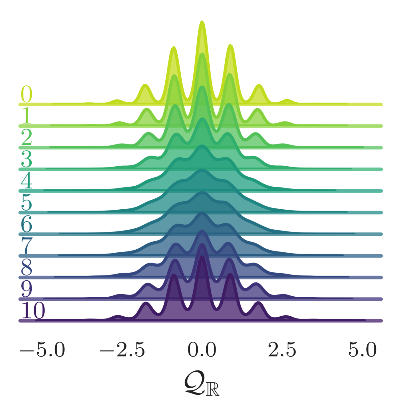
Introduce an annealing schedule during the training phase:

(varied slowly)

e.g. \( \{0.1, 0.2, \ldots, 0.9, 1.0\}\)

(increasing)

p_{t}(x)\propto e^{-\gamma_{t}S(x)},\quad\text{for}\quad t=0, 1,\ldots, N

Target distribution becomes:

For \(\|\gamma_{t}\| < 1\), this helps to rescale (shrink) the energy barriers between isolated modes
- Allows our sampler to explore previously inaccessible regions of the target distribution

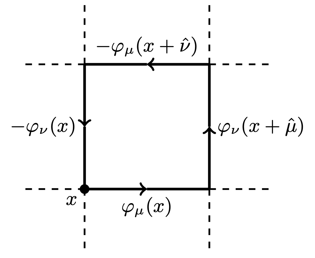
Wilson action:

S(\varphi)=\sum_{P}1-\cos\varphi_{P}

\varphi_{P} = \varphi_{\mu}(x) + \varphi_{\nu}(x+\hat{\mu}) - \varphi_{\mu}(x+\hat{\nu}) - \varphi_{\nu}(x)

Topological charge:

continuous, differentiable

discrete, hard to work with

\left\lfloor\varphi_{P}\right\rfloor = \varphi_{P} - 2\pi\left\lfloor\frac{\varphi_{P}+\pi}{2\pi}\right\rfloor

\mathcal{Q}_{\mathbb{Z}} = \frac{1}{2\pi}\sum_{P}\left\lfloor\varphi_{P}\right\rfloor\hspace{6pt} \in\mathbb{Z}

\mathcal{Q}_{\mathbb{R}} = \frac{1}{2\pi}\sum_{P}\sin\varphi_{P}\in\mathbb{R}

Link variables:

U_{\mu}(x) = e^{i\varphi_{\mu}(x)} \in U(1)

x_{\mu}(n) \in [-\pi,\pi]

Lattice Gauge Theory

We maximize the expected squared charge difference:

Loss function: \(\mathcal{L}(\theta)\)

\delta \mathcal{Q}_{\mathbb{R}}^{2}(\xi',\xi) \equiv \left(\mathcal{Q}_{\mathbb{R}}(x') - \mathcal{Q}_{\mathbb{R}}(x)\right)^{2}

\mathcal{L}(\theta) = \mathbb{E}_{p(\xi)}\left[-\delta\mathcal{Q}^{2}_{\mathbb{R}}(\xi',\xi)\cdot A(\xi'|\xi)\right]

A(\xi'|\xi) = \min\left\{1, \frac{p(\xi')}{p(\xi)} \left|\frac{\partial\xi'}{\partial\xi^{T}}\right|\right\}

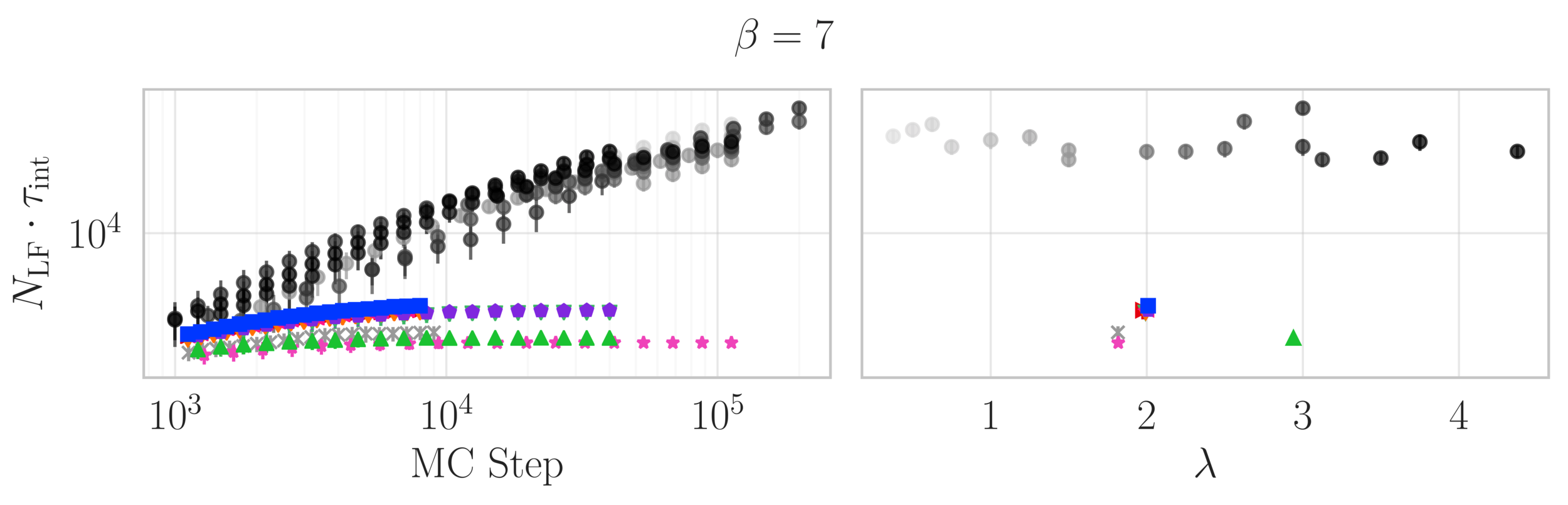
Results

We maximize the expected squared charge difference:

\delta \mathcal{Q}_{\mathbb{R}}^{2}(\xi',\xi) \equiv \left(\mathcal{Q}_{\mathbb{R}}(x') - \mathcal{Q}_{\mathbb{R}}(x)\right)^{2}

\mathcal{L}(\theta) = \mathbb{E}_{p(\xi)}\left[-\delta\mathcal{Q}^{2}_{\mathbb{R}}(\xi',\xi)\cdot A(\xi'|\xi)\right]

A(\xi'|\xi) = \min\left\{1, \frac{p(\xi')}{p(\xi)} \left|\frac{\partial\xi'}{\partial\xi^{T}}\right|\right\}

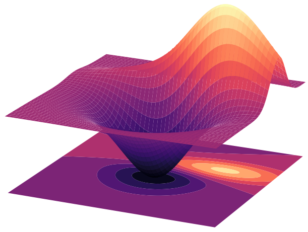
Interpretation

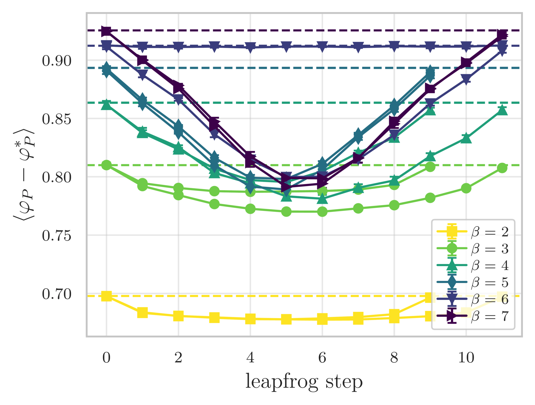
Look at how different quantities evolve over a single trajectory
- See that the sampler artificially increases the energy during the first half of the trajectory (before returning to original value)

Leapfrog step

variation in the avg. plaquette

continuous topological charge

shifted energy

GMM: Autocorrelation

L2HMC

HMC

Lattice Gauge Theory

Topological Loss Function:

\ell_{\theta}(\xi^{\prime}, \xi, A(\xi^{\prime}|\xi)) = -\frac{1}{a^{2}}A(\xi^{\prime}|\xi)\cdot \delta_{\mathcal{Q}_{\mathbb{R}}}(\xi^{\prime}, \xi)

\delta_{\mathcal{Q}_{\mathbb{R}}}(\xi^{\prime}, \xi) \equiv \left(\mathcal{Q}_{\mathbb{R}}^{\prime} - \mathcal{Q}_{\mathbb{R}}\right)^{2}

= \left(\mathcal{Q}_{\mathbb{R}}(\xi^{\prime}) - \mathcal{Q}_{\mathbb{R}}(\xi)\right)^{2}

\(A(\xi^{\prime}|\xi) = \) "acceptance probability"

where:

Lattice Gauge Theory

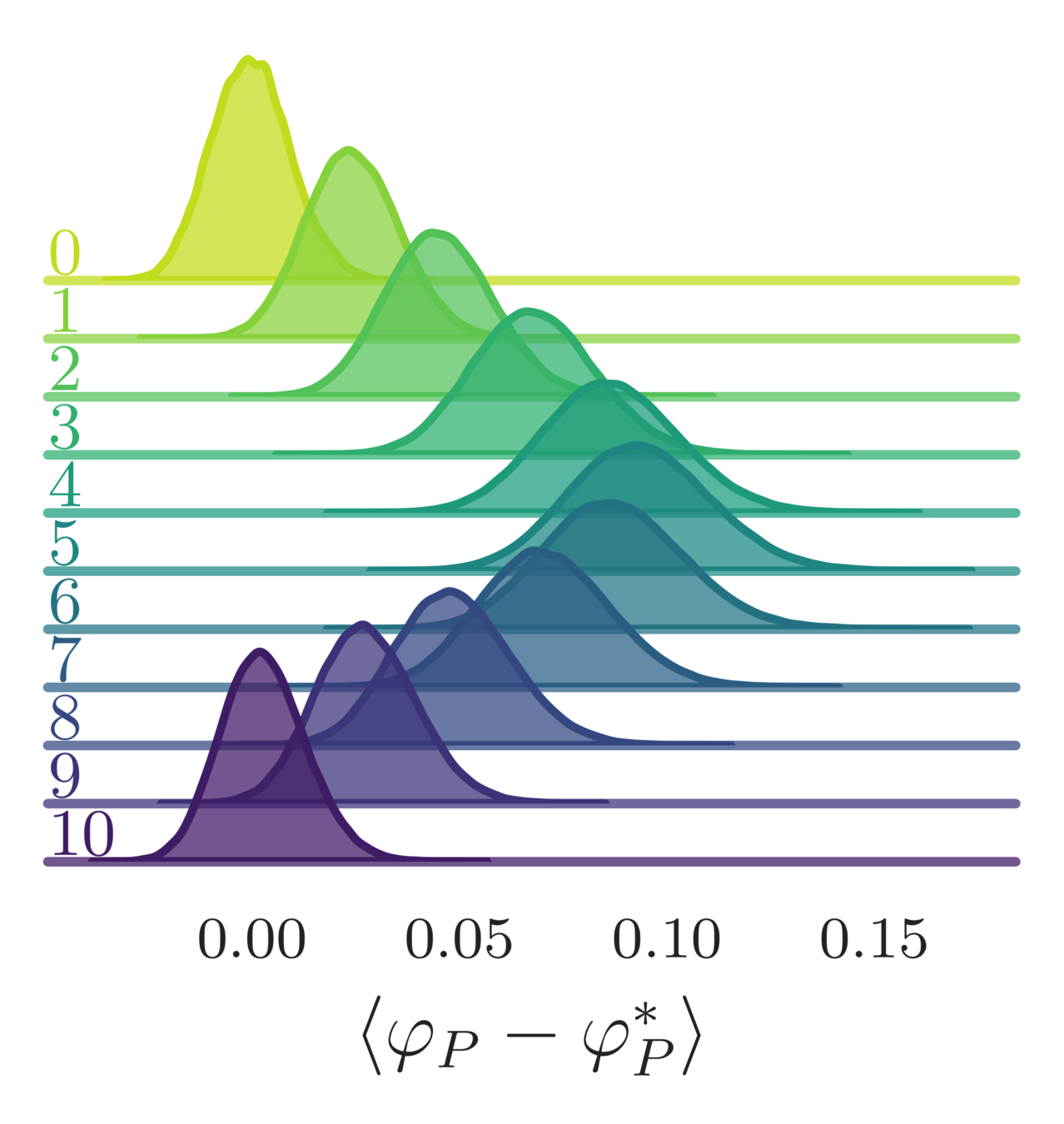
Variation in the average plaquette, \(\langle\varphi_{P}-\varphi^{*}\rangle\)
- where \(\varphi^{*} = I_{1}(\beta)/I_{0}(\beta)\) is the exact (\(\infty\)-volume) result

leapfrog step

(MD trajectory)

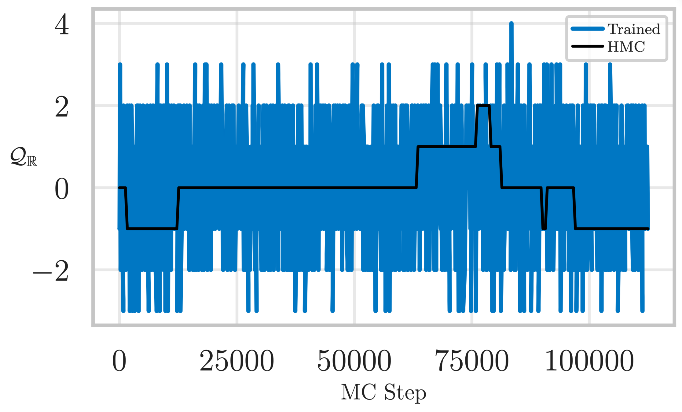
Topological charge history

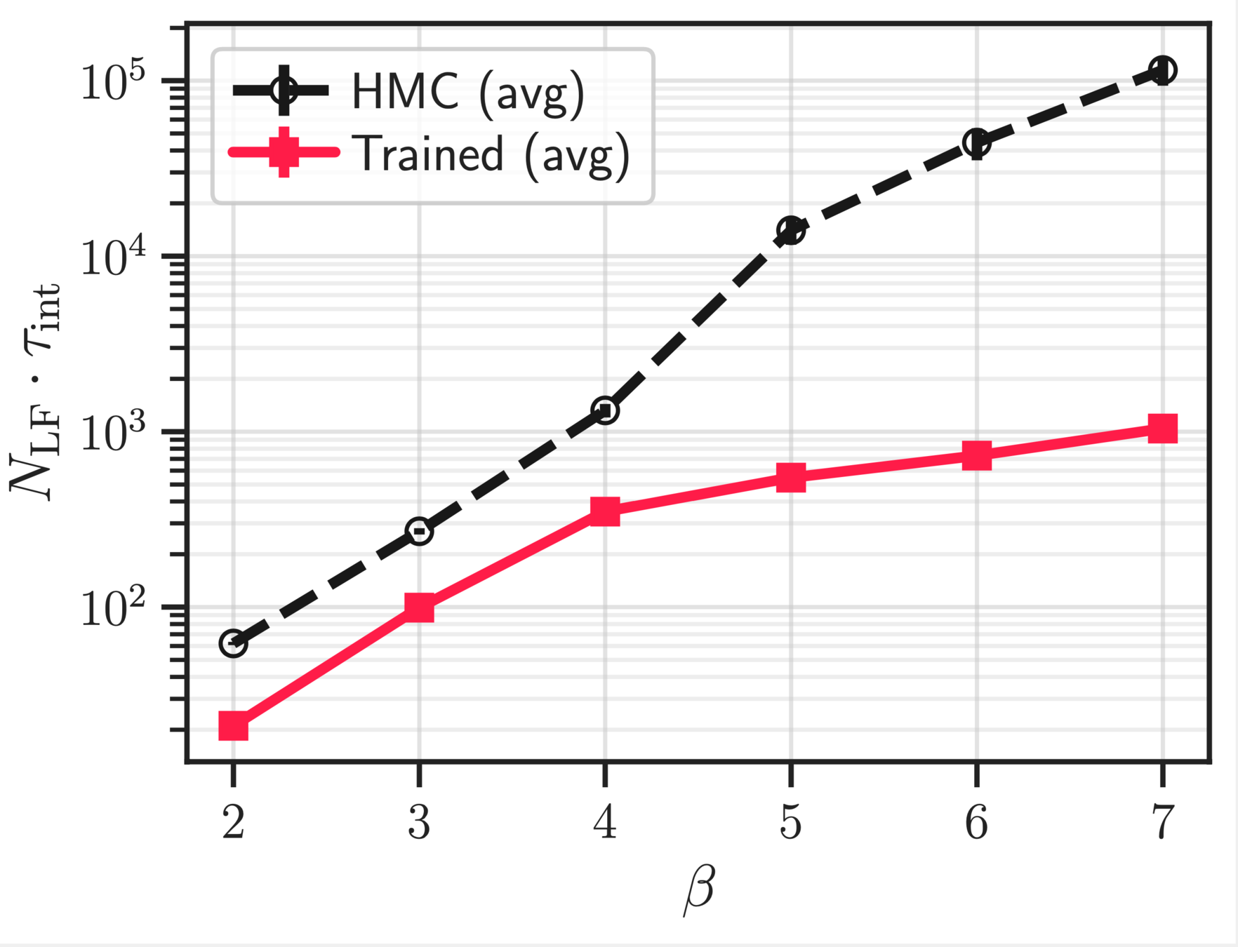
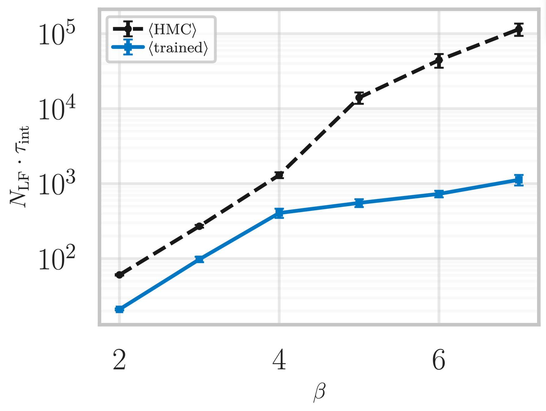
~ cost / step

continuum limit

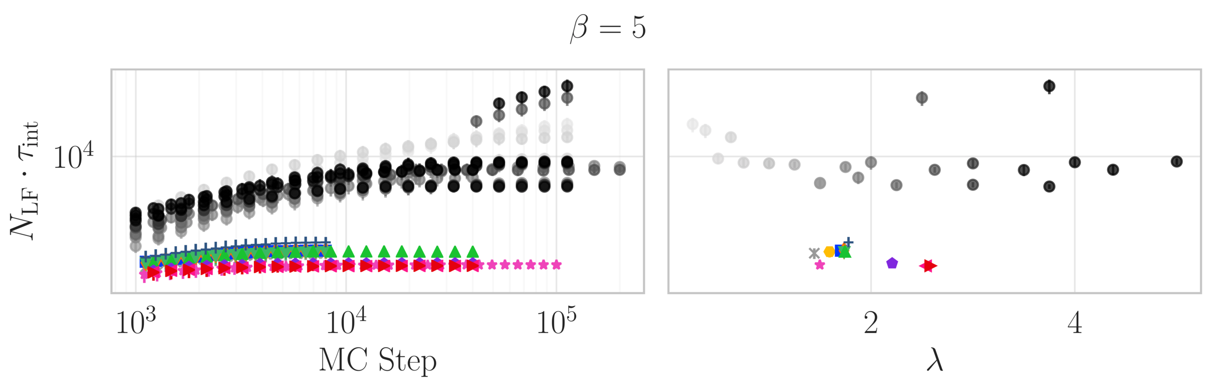
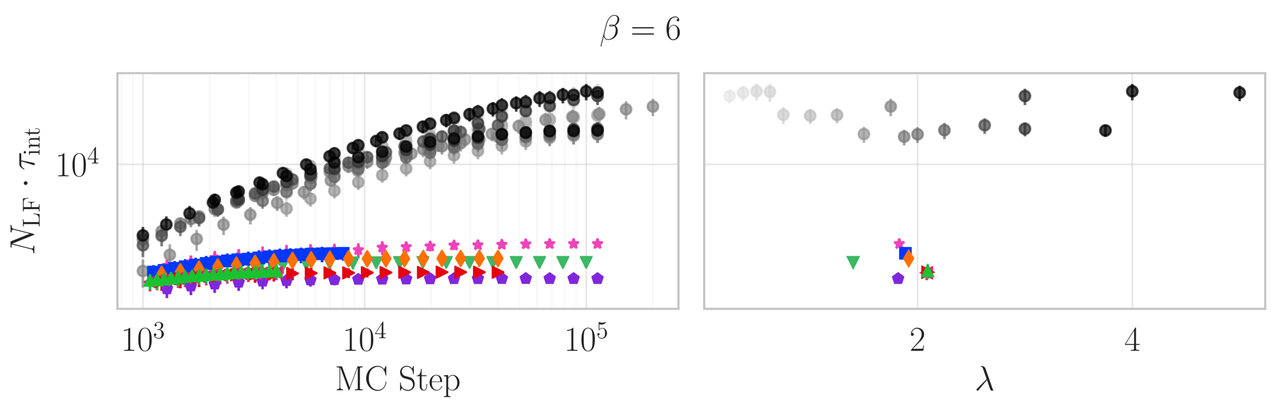
Estimate of the Integrated autocorrelation time of \(\mathcal{Q}_{\mathbb{R}}\)

Generalized Leapfrog Update

Jacobian:

\(\left|\frac{\partial v''_{k}}{\partial v_{k}}\right|=\exp\left(\frac{1}{2}\varepsilon^{k}_{v} s_{v}^{k}(\zeta_{v_{k}})\right)\), \(\left|\frac{\partial x''_{k}}{\partial x_{k}}\right|=\exp\left(\varepsilon^{k}_{v} s_{v}^{k}(\zeta_{v_{k}})\right)\)

Update complementary indices determined by and

L2HMC: Generalized Leapfrog

Main idea

Introduce \((s_{x}, t_{x}, q_{x})\), \((s_{v}, t_{v}, q_{v})\) into the leapfrog updates, which are parameterized by weights \(\theta\) in a neural network.
Introduce a binary direction variable, \(d\sim\mathcal{U}(+,-)\)
Denote a complete state by \(\xi = (x, v, d)\), with target distribution \(p(\xi)\):

p(\xi) = p(x, v, d) = p(x)\cdot p(v)\cdot p(d)

Jacobian:

Text

Example: GMM \(\in\mathbb{R}^{2}\)

\(A(\xi',\xi)\) = acceptance probability

\(A(\xi'|\xi)\cdot\delta(\xi',\xi)\) = avg. distance

Note:

Define the squared jump distance:

\delta(\xi^{\prime}, \xi) = \|x^{\prime} - x\|^{2}_{2}

Maximize expected squared jump distance:

\ell_{\theta}\left[\xi^{\prime}, \xi, A(\xi^{\prime}|\xi)\right] = \frac{a^{2}}{A(\xi^{\prime}|\xi)\cdot\delta(\xi^{\prime},\xi)} - \frac{A(\xi^{\prime}|\xi)\cdot\delta(\xi^{\prime},\xi)}{a^{2}}

Encourages large moves

Penalizes small moves

\mathcal{L}_{\theta}\left(\theta\right) \equiv \mathbb{E}_{p(\xi)}\left[A(\xi'|\xi)\cdot \delta(\xi',\xi)\right]

HMC

L2HMC

where:

L2HMC: Generalized Leapfrog

x^{\prime}_{k} = \Lambda^{+}_{k}(x_{k};\zeta_{x_{k}})

Generalized \(x\)-update:

\zeta_{x_{k}}\equiv \big(\quad\odot x_{k}, \partial_{x}S(x_{k})\big),

\bar{m}_{t}

\overbrace{\hspace{75px}}

Momentum (\(v_{k}\)) scaling

(\(v\)) independent

Gradient \(\partial_{x}S(x_{k})\) scaling

\overbrace{\hspace{100px}}

\overbrace{\hspace{30px}}

Translation

(\(m_{t}\)\(\odot x\)) independent

Neural Networks

\zeta_{v_{k}}\equiv \big(x_{k}, \partial_{x}S(x_{k})\big)

Generalized \(v\)-update:

v^{\prime}_{k} = \Gamma^{+}_{k}(v_{k};\zeta_{v_{k}} )

m_{t}

\bar{m}_{t}

= \mathbb{1}

(masks)

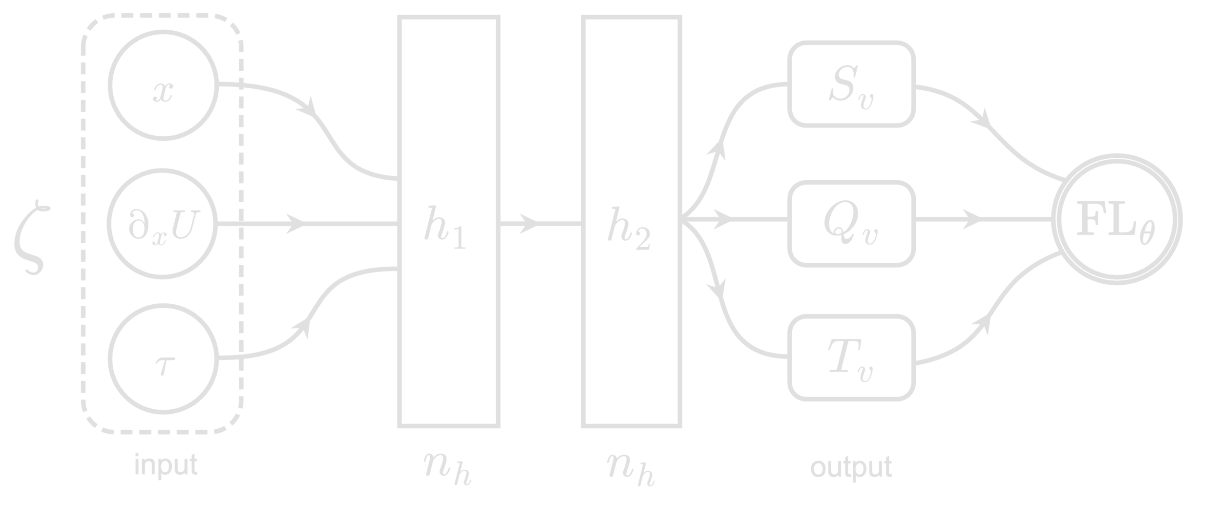
Network Architecture

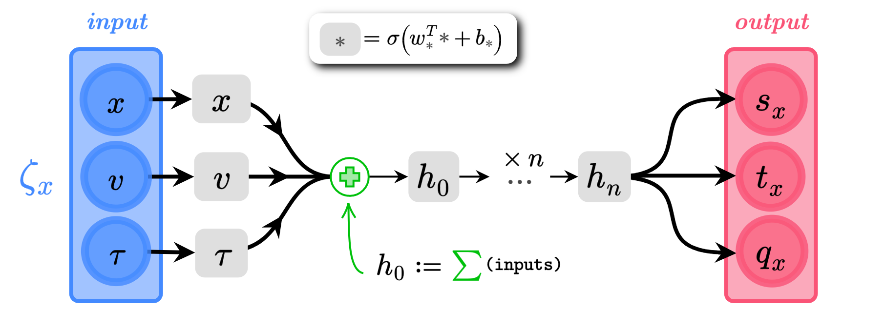
s_{x} = \alpha_{s}\tanh(w^{T}_{s} h_{n} + b_{s})

q_{x} = \alpha_{q}\tanh(w^{T}_{q} h_{n} + b_{q})

t_{x} = w_{t}^{T} h_{n} + b_{t} \in \mathbb{R}^{n}

(\(\alpha_{s}, \alpha_{q}\) are trainable parameters)

\(x\), \(v\) \(\in \mathbb{R}^{n}\)

\(s_{x}\),\(q_{x}\),\(t_{x}\) \(\in \mathbb{R}^{n}\)

4096

8192

1024

2048

512

Scaling test: Training

\(4096 \sim 1.73\times\)

\(8192 \sim 2.19\times\)

\(1024 \sim 1.04\times\)

\(2048 \sim 1.29\times\)

\(512\sim 1\times\)

Scaling test: Training

\(8192\sim \times\)

4096

1024

2048

512

Scaling test: Inference

L2HMC: Generalized Leapfrog

Define (\(v\)-independent): \(\zeta_{v_{k}} \equiv (x_{k}, \partial_{x}S(x_{k}), \tau(k))\)

v^{\prime}_{k} \equiv \Gamma^{+}_{k}(v_{k};\zeta_{v_{k}}) = v_{k}\odot \exp\left(\frac{\varepsilon^{k}_{v}}{2}s^{k}_{v}(\zeta_{v_{k}})\right) - \frac{\varepsilon^{k}_{v}}{2}\left[\partial_{x}S(x_{k})\odot\exp\left(\varepsilon^{k}_{v}q^{k}_{v}(\zeta_{v_{k}})\right) + t^{k}_{v}(\zeta_{v_{k}})\right]

\overbrace{\hspace{85px}}

Momentum scaling

Gradient scaling

\overbrace{\hspace{30px}}

Translation

x^{\prime}_{k} \equiv \Lambda^{+}_{k}(x_{k};\zeta_{x_{k}}) = x_{k}\odot\exp\left(\varepsilon^{k}_{x}s^{k}_{x}(\zeta_{x_{k}})\right) + \varepsilon^{k}_{x}\left[v^{\prime}_{k}\odot\exp\left(\varepsilon^{k}_{x}q^{k}_{x}(\zeta_{x_{k}})\right)+t^{k}_{x}(\zeta_{x_{k}})\right]

\overbrace{\hspace{105px}}

Introduce generalized \(v\)-update, \(\Gamma^{+}_{k}(v_{k};\zeta_{v_{k}})\):

Define (\(x\)-independent): \(\zeta_{x_{k}} = (x_{k}, v_{k}, \tau(k))\)

Introduce generalized \(x\)-update, \(\Lambda^{+}_{k}(x_{k};\zeta_{x_{k}})\)

momentum

position

L2HMC: Modified Leapfrog

Split the position, \(x\), update into two sub-updates:
- Introduce a binary mask \(m^{t} \in\{0, 1\}^{n}\) and its complement \(\bar{m}^{t}\).
- \(m^{t}\) is drawn uniformly from the set of binary vectors satisfying \(\sum_{i=1}^{n}m_{i}^{t} = \lfloor{\frac{n}{2}\rfloor}\) (i.e. half of the entries of \(m^{t}\) are 0 and half are 1.)

Introduce a binary direction variable \(d \in \{-1, 1\}\), drawn from a uniform distribution.
- Denote the complete augmented state as \(\xi \equiv (x, v, d)\).

(forward direction, \(d = +1\))

v_{k}^{\prime} = v\odot\exp\left(\frac{\varepsilon^{k}_{v}}{2}s^{k}_{v}(\zeta_{v_{k}})\right) - \frac{\varepsilon^{k}_{v}}{2}\left[\partial_{x}U(x)\odot\exp(\varepsilon^{k}_{v} q^{k}_{v}(\zeta_{v_{k}})) + t^{k}_{v}(\zeta_{v_{k}})\right]

x_{k}^{\prime} = x^{k}_{\bar{m}^{t}} + m^{t}\odot\left[x^{k}\odot \exp(\varepsilon^{k}_{x} s^{k}_{x}(\zeta_{x_{k}})) + \varepsilon^{k}_{x}\left(v^{\prime} \odot\exp(\varepsilon^{k}_{x} q^{k}_{x}(\zeta_{x_{k}})) + t^{k}_{x}(\zeta_{x_{k}})\right)\right]

x_{k}^{\prime\prime} = x_{\bar{m}^{t}}^{\prime} + \bar{m}^{t}\odot\left[x^{\prime}\odot \exp(\varepsilon S_{x}(\zeta_{3})) + \varepsilon\left(v^{\prime} \odot\exp(\varepsilon Q_{x}(\zeta_{3})) + T_{x}(\zeta_{3})\right)\right]

v_{k}^{\prime\prime} = v^{\prime}\odot\exp\left(\frac{\varepsilon}{2}S_{v}(\zeta_{4})\right) - \frac{\varepsilon}{2}\left[\partial_{x}U(x^{\prime\prime})\odot\exp(\varepsilon Q_{v}(\zeta_{4})) + T_{v}(\zeta_{4})\right]

\zeta_{1} = (x, \partial_{x}U(x), t)

\zeta_{2} = (x_{\bar{m}^{t}}, v, t)

\zeta_{3} = (x^{\prime}_{m^{t}}, v, t)

\zeta_{4} = (x^{\prime\prime}, \partial_{x}U(x^{\prime\prime}), t)

\overbrace{\hspace{35px}}

Momentum scaling

\overbrace{\hspace{43px}}

Gradient scaling

\overbrace{\hspace{5px}}

Translation

inputs

L2HMC: Modified Leapfrog

Writing the action of the new leapfrog integrator as an operator \(\mathbf{L}_{\theta}\), parameterized by \(\theta\).

Applying this operator \(M\) times successively to \(\xi\):

\mathbf{L}_{\theta} = \mathbf{L}_{\theta}(x, v, d) = \left(x^{{\prime\prime}^{\times M}}, v^{{\prime\prime}^{\times M}}, d\right)

The "flip" operator \(\mathbf{F}\) reverses \(d\): \(\mathbf{F}\xi = (x, v, -d)\).

Write the complete dynamics step as:

\mathbf{FL}_{\theta} \xi = \xi^{\prime}

(trajectory length)

L2HMC: Accept/Reject

Fortunately, the Jacobian can be computed efficiently, and only depends on \(S_{x}, S_{v}\) and all the state variables, \(\zeta_{i}\).

This has the effect of deforming the energy landscape:

\mathcal{J}

Accept the proposed configuration, \(\xi^{\prime}\) with probability:

\(A(\xi^{\prime}|\xi) = \min{\left(1, \frac{p(\mathbf{FL}_{\theta}\xi)}{p(\xi)}\left|\frac{\partial\left[\mathbf{FL}\xi\right]}{\partial\xi^{T}}\right|\right)}\)

\(|\mathcal{J}| \neq 1\)

Unlike HMC,

L2HMC: Loss function

\ell_{\lambda}\left(\xi, \xi^{\prime}, A(\xi^{\prime}|\xi)\right) = \frac{\lambda^{2}}{\delta(\xi, \xi^{\prime})A(\xi^{\prime}|\xi)} - \frac{\delta(\xi, \xi^{\prime})A(\xi^{\prime}|\xi)}{\lambda^{2}}

\underbrace{\hspace{38px}}

Encourages typical moves to be large

\overbrace{\hspace{38px}}

Penalizes sampler if unable to move effectively

scale parameter

"distance" between \(\xi, \xi^{\prime}\): \(\delta(\xi, \xi^{\prime}) = \|x - x^{\prime}\|^{2}_{2}\)

Idea: MINIMIZE the autocorrelation time (time needed for samples to be independent).
- Done by MAXIMIZING the "distance" traveled by the integrator.

Note:

\(\delta \times A = \) "expected" distance

L2HMC: \(U(1)\) Lattice Gauge Theory

U_{\mu}(i) = e^{i \phi_{\mu}(i)} \in U(1)

-\pi < \phi_{\mu}(i) \leq \pi

\beta S = \beta \sum_{P}\left(1 - \cos(\phi_{P})\right)

Wilson action:

\phi_{P} \equiv \phi_{\mu\nu}(i)\\

= \phi_{\mu}(i) + \phi_{\nu}(i + \hat{\mu})- \phi_{\mu}(i+\hat{\nu}) - \phi_{\nu}(i)

where:

L2HMC: \(U(1)\) Lattice Gauge Theory

U_{\mu}(i) = e^{i \phi_{\mu}(i)} \in U(1)

-\pi < \phi_{\mu}(i) \leq \pi

\beta S = \beta \sum_{P}\left(1 - \cos(\phi_{P})\right)

Wilson action:

\phi_{P} \equiv \phi_{\mu\nu}(i)\\

= \phi_{\mu}(i) + \phi_{\nu}(i + \hat{\mu})- \phi_{\mu}(i+\hat{\nu}) - \phi_{\nu}(i)

where:

L2HMC

HMC

L2HMC

HMC

Thanks for listening!

Interested?

github.com/saforem2/l2hmc-qcd

Machine Learning in Lattice QCD

Sam Foreman

02/10/2020

Network Architecture

Build model,

initialize network

Run dynamics, Accept/Reject

Calculate

Backpropagate

Finished

training?

Save trained

model

Run inference

on saved model

\ell_{\lambda}(\theta)

Train step

Hamiltonian Monte Carlo (HMC)

Integrating Hamilton's equations allows us to move far in state space while staying (roughly) on iso-probability contours of \(p(x, v)\)

Integrate \(H(x, v)\):

\(t \longrightarrow t + \varepsilon\)

Project onto target parameter space \(p(x, v) \longrightarrow p(x)\)

\(v \sim p(v)\)

Markov Chain Monte Carlo (MCMC)

Goal: Generate an ensemble of independent samples drawn from the desired target distribution \(p(x)\).

This is done using the Metropolis-Hastings accept/reject algorithm:

Given:
- Initial distribution, \(\pi_{0}\)
- Proposal distribution, \(q(x^{\prime}|x)\)
Update:
1. Sample \(x^{\prime} \sim q(\cdot | x)\)
2. Accept \(x^{\prime}\) with probability \(A(x^{\prime}|x)\)

A(x^{\prime}|x) = \min\left[1, \frac{p(x^{\prime})q(x|x^{\prime})}{p(x)q(x^{\prime}|x)}\right] = \min\left[1, \frac{p(x^{\prime})}{p(x)}\right]

if \(q(x^{\prime}|x) = q(x|x^{\prime})\)

\longrightarrow

HMC: Leapfrog Integrator

Integrate Hamilton's equations numerically using the leapfrog integrator.

The leapfrog integrator proceeds in three steps:

\dot x_{i} = \frac{\partial\mathcal{H}}{\partial v_{i}} = v_i

\dot v_{i} =-\frac{\partial\mathcal{H}}{\partial x_{i}} = -\frac{\partial U}{\partial x_{i}}

Update momenta (half step):

Update position (full step):

Update momenta (half step):

(1.)

(2.)

(3.)

(t \longrightarrow t + \frac{\varepsilon}{2})

(t \longrightarrow t + \varepsilon)

(t + \frac{\varepsilon}{2} \longrightarrow t + \varepsilon)

v(t + \frac{\varepsilon}{2}) = v(t) - \frac{\varepsilon}{2}\partial_{x} U(x(t))

x(t + \varepsilon) = x(t) + \varepsilon v(t+\frac{\varepsilon}{2})

v(t+\varepsilon) = v(t+\frac{\varepsilon}{2}) - \frac{\varepsilon}{2}\partial_{x}U(x(t+\varepsilon))

Issues with MCMC

Need to wait for the chain to "burn in" (become thermalized)

Nearby configurations on the chain are correlated with each other.
- Multiple steps needed to produce independent samples ("mixing time")
  - Measurable via integrated autocorrelation time, \(\tau^{\mathrm{int}}_{\mathcal{O}}\)

Smaller \(\tau^{\mathrm{int}}_{\mathcal{O}}\longrightarrow\) less computational cost!

correlated!

burn-in

\underbrace{\hspace96px}

\sim p(x)

\overbrace{\hspace 72px}

L2HMC: Learning to HMC

L2HMC generalizes HMC by introducing 6 new functions, \(S_{\ell}, T_{\ell}, Q_{\ell}\), for \(\ell = x, v\) into the leapfrog integrator.

Given an analytically described distribution, L2HMC provides a statistically exact sampler, with highly desirable properties:

Fast burn-in.
Fast mixing.

Ideal for lattice QCD due to critical slowing down!

Idea: MINIMIZE the autocorrelation time (time needed for samples to be independent).
- Can be done by MAXIMIZING the "distance" traveled by the integrator.

HMC: Leapfrog Integrator

Write the action of the leapfrog integrator in terms of an operator \(L\), acting on the state \(\xi \equiv (x, v)\):

\mathbf{L}\xi \equiv \mathbf{L}(x, v)\equiv (x^{\prime}, v^{\prime})

\mathbf{F}\xi \equiv \mathbf{F}(x, v) \equiv (x, -v)

The acceptance probability is then given by:

Introduce a "momentum-flip" operator, \(\mathbf{F}\):

A\left(\xi^{\prime}|\xi\right) = \min\left(1, \frac{p(\xi^{\prime})}{p(\xi)}\left|\frac{\partial\left[\xi^{\prime}\right]}{\partial\xi^{T}}\right|\right)

Determinant of the Jacobian, \(\|\mathcal{J}\|\)

(for HMC)

L2HMC: Generalized Leapfrog

Define (\(v\)-independent): \(\zeta_{v_{k}} \equiv (x_{k}, \partial_{x}S(x_{k}), \tau(k))\)

\overbrace{\hspace{85px}}

Momentum scaling

Gradient scaling

\overbrace{\hspace{30px}}

Translation

\overbrace{\hspace{105px}}

Introduce generalized \(v\)-update, \(\Gamma^{+}_{k}(v_{k};\zeta_{v_{k}})\):

For \(\zeta_{x_{k}} = (x_{k}, v_{k}, \tau(k))\)

And the generalized \(x\)-update, \(\Lambda^{+}_{k}(x_{k};\zeta_{x_{k}})\)

momentum

position

Copy of DLHMC_MIT_lattice

By Sam Foreman

Copy of DLHMC_MIT_lattice

Machine Learning in Lattice QCD

Sam Foreman

saforem2

Deep Learning HMC

Building Topological Samplers for Lattice QCD

MCMC in Lattice QCD

Markov Chain Monte Carlo (MCMC)

Issues with MCMC

Hamiltonian Monte Carlo (HMC)

HMC: Leapfrog Integrator

Hamilton's Eqs:

Hamiltonian:

\(N_{\mathrm{LF}}\) leapfrog steps:

Leapfrog Integrator

HMC: Issues

Leapfrog Layer

Leapfrog Layer

L2HMC: Generalized Leapfrog

Leapfrog Layer

Example: GMM \(\in\mathbb{R}^{2}\)

Training Algorithm

Annealing Schedule

Lattice Gauge Theory

Loss function: \(\mathcal{L}(\theta)\)

Results

Interpretation

GMM: Autocorrelation

L2HMC

HMC

Lattice Gauge Theory

Lattice Gauge Theory

Generalized Leapfrog Update

L2HMC: Generalized Leapfrog

Example: GMM \(\in\mathbb{R}^{2}\)

L2HMC: Generalized Leapfrog

Network Architecture

Scaling test: Training

Scaling test: Training

Scaling test: Training

Scaling test: Inference

L2HMC: Generalized Leapfrog

L2HMC: Modified Leapfrog

L2HMC: Modified Leapfrog

L2HMC: Accept/Reject

L2HMC: Loss function

L2HMC: \(U(1)\) Lattice Gauge Theory

Wilson action:

L2HMC: \(U(1)\) Lattice Gauge Theory

Wilson action:

L2HMC

HMC

L2HMC

HMC

Thanks for listening!

Machine Learning in Lattice QCD

Sam Foreman

Network Architecture

Hamiltonian Monte Carlo (HMC)

HMC: Leapfrog Integrator

Update momenta (half step):

Update position (full step):

Update momenta (half step):

Issues with MCMC

Smaller \(\tau^{\mathrm{int}}_{\mathcal{O}}\longrightarrow\) less computational cost!

L2HMC: Learning to HMC

HMC: Leapfrog Integrator

L2HMC: Generalized Leapfrog

Copy of DLHMC_MIT_lattice

More from Sam Foreman