A Gentle Introduction to Machine Learning and Neural Networks
Sean Meling Murray,
Department of Mathematics,
University of Bergen

Sources: New York Post, Futurism, VICE Motherboard, The Conversation, The Verge

Machine learning gives computers the ability to learn from data without being explicitly programmed to do so.
Algorithms allow us to build models that make data-driven predictions about the stuff we're interested in.
Wikipedia:
Regression
Typically used when we want our model to predict a continuous numerical value.
Classification
Typically used when we want our model to classify an event or a thing into one of K categories.
E.g. How much is my apartment worth given size, number of rooms, etc.?
E.g. Given today's housing market, will I be able to sell my apartment (yes or no)?
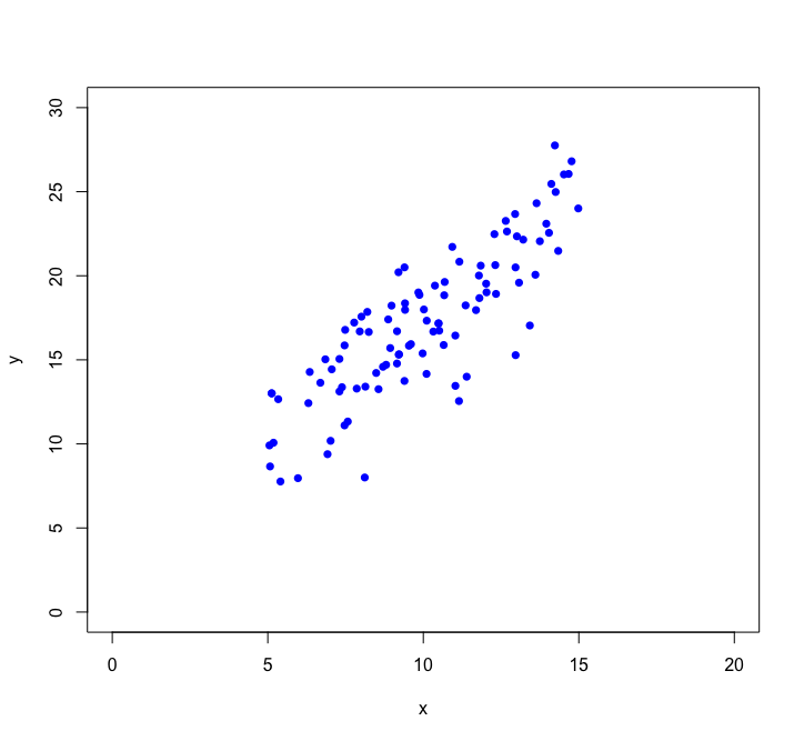
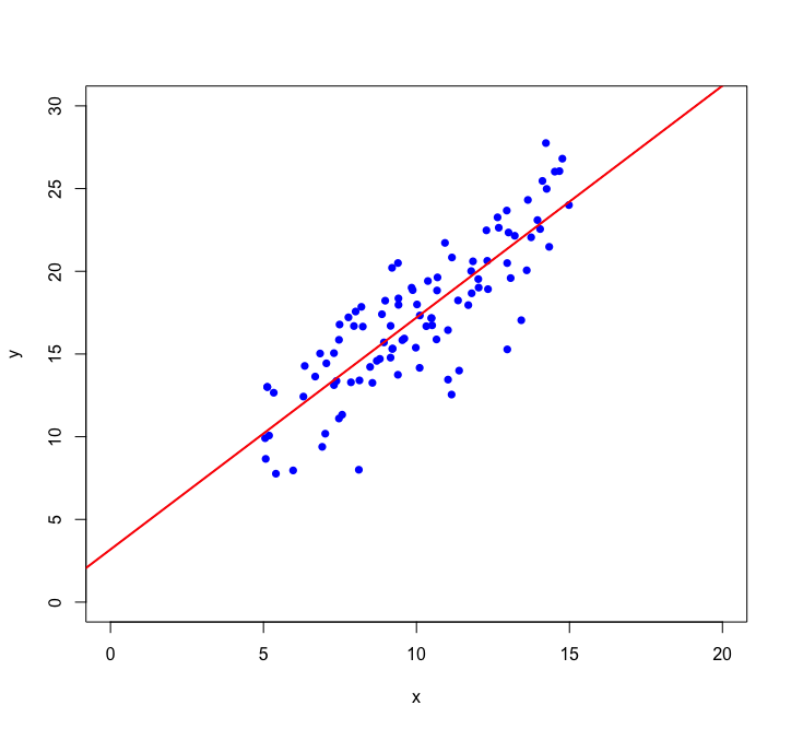
Let's look closer at linear regression:
Using we want to find the straight line that best fits the data:
\hat{y} = \hat{w}_0 + \hat{w}_1x
This is
our model
intercept
slope
parameters
input aka. features, i.e. properties of the thing we are trying to predict
y_i \approx w_0 + w_1x_i
output
(x_i, y_i)
Supervised
We compare our model's prediction to a known label or value and try to make the prediction error as small as possible.
Unsupervised
We try to identify meaningful patterns in unlabelled data. In other words, we let the data speak for itself.
Source: Tango with Code
Source: Sagar Sharma, towardsdatascience.com
C(y,\hat{y}) = \frac{1}{2N} \sum_{i=1}^N (y_i - \hat{y}_i)^2
We want to minimize the prediction errors:
Mean squared error (MSE)
Using the input-output pairs in our data, which combination of weight settings gives us the lowest value of the cost function?
Cost
True value
Prediction
Training
, optimizing
(x_i, y_i)
learning
,
\frac{\partial C}{\partial w_0} = 0
\frac{\partial C}{\partial w_1} = 0
Solve:
Let's visualize the regression line a little differently...
y_i = w_0+w_1x_i
w_0
w_1
1
x_i
\sum{}
y_i
y_i
=
w_0
+
w_1
x_i
1
Intercept
Feature
Let's call these circles neurons!
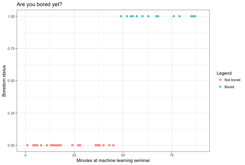
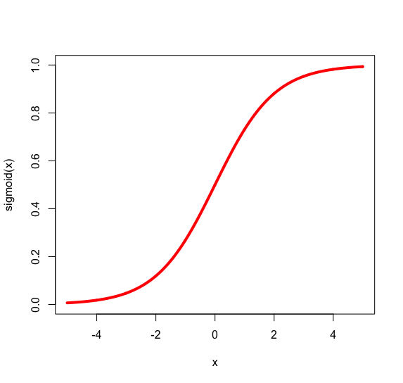
What if we want to model a non-linear relationship?
y_i = \frac{1}{1+e^{-(w_0+w_1x_i)}}
w_0
w_1
1
x_i
\sum{}|\sigma
y_i
\sigma_1(input) = \frac{1}{1+e^{-input}}
y_i
\sigma_2(\sigma_1(input)) =
\begin{cases}
\text{bored if }\sigma_1(input)>0.5\\
\text{not bored otherwise}
\end{cases}
Thresholding
1
x_n
\sum{}|\sigma
y
1
\sum{}|\sigma
We call the weighted sum of inputs the activation of the neuron. The non-linear transformation is called the activation function.
Neural network!
weights
weights
y
=
\sigma_2
\sigma_1
\text{W}_1x
(
(
)
)
\text{w}_2^\text{T}
Composition of non-linear functions!
\text{W}_1
\text{w}_2
Network architecture
The number of neurons in a layer is it's width.
Many layers results in a deep model, and is why we call it deep learning.
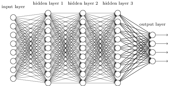
Image credit: KDNuggets
The number of layers in a network is it's depth.
How does a neural network learn?
1. Backpropagation
2. Gradient descent
1. Backpropagation
Check out 3blue1brown on YouTube
Backprop algorithm calculates the gradients of cost function wrt. the networks weights using the chain rule!

Iteratively nudge the weights in the direction where cost decreases the most, i.e. the negative of the gradient calculated in step 1.
C(y,\hat{y})
\hat{y}_i = \hat{w}_0 + \hat{w}_1x_i
Source: Tango with Code
2. Gradient descent
Deep Learning models
Convolutional neural networks
Image recognition and object detection:
https://github.com/shaoanlu/Udacity-SDCND-Vehicle-Detection
Recurrent neural networks
Natural language processing:
http://karpathy.github.io/2015/05/21/rnn-effectiveness/
Reinforcement learning
Building software agents that
learn by reacting to the environment:

From the documentary AlphaGo
Google DeepMind
Generative adversarial networks
Pairs of networks that
generate images and other types of data:
https://github.com/junyanz/CycleGAN
Thanks!
A Gentle Introduction to Machine Learning and Neural Networks
By Sean Meling Murray
A Gentle Introduction to Machine Learning and Neural Networks
Presentation held at the first machine learning seminar arranged by the Western Norway University of Applied Sciences, the University of Bergen and Haukeland University Hospital. See https://mmiv.no/upcoming/ for upcoming events.
