
Methods for large-scale modeling and simulation
Sebastian Hörl
Spring 2023
Université Gustave Eiffel
Overview
- Lectures covering example sand methods in large-scale transport planning making use of open data sources
- Project work on the assessment of the Grand Paris Express
- Work in groups of ~5 students
- Exchange necessary between individual groups
- Assessment
- Project presentation at the end of the course
- Short report on the project
Timeline
- Lectures
- 10/01 8h30: Examples of large-scale models in transportation
- 10/01 10h45: Modeling methods I
- 13/01 14h00: Modeling methods II
- 13/01 16h45: Introduction to the student project
- Project work
- 27/01 14h00 + 16h45: Intermediate results
- 09/02 14h00 + 16h45: Exchange with other groups
- 23/02 14h00 + 16h45: Final presentation
2 weeks
2 weeks
2 weeks
Timeline
- Lectures
- 10/01 8h30: Examples of large-scale models in transportation
- 10/01 10h45: Modeling methods I
- 13/01 14h00: Modeling methods II
- 13/01 16h45: Introduction to the student project
- Project work
- 27/01 14h00 + 16h45: Intermediate results
- 09/02 14h00 + 16h45: Exchange with other groups
- 23/02 14h00 + 16h45: Final presentation
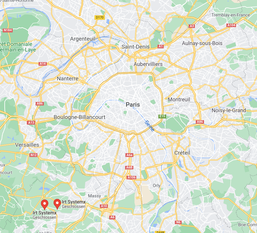
IRT SystemX
- Public/private research institute situated in Paris
- Focus on fostering digital transition in a range of fields from transport, cybersecurity to circular economy
- Transferring research results and tools into active application by development and provision of industry platforms
- Various collaborative projects with multiple French companies (Renault, SNCF, ...) and academic partners (Université Paris Saclay, CentraleSupélec, Université Gustave Eiffel)
- Participation in European projects
http://www.loc.gov/pictures/item/2016800172/
The street in 1900
The street today
https://commons.wikimedia.org/wiki/File:Atlanta_75.85.jpg
- Autonomous Mobility
- Mobility as a Service
- Mobility on Demand
- Electrification
- Aerial Mobility
Julius Bär / Farner
The street of tomorrow?
I. Transport simulation
Classic transport planning
- Zones
- Flows
- Peak hours
- User groups
Aggregated
Agent-based models


0:00 - 8:00
08:30 - 17:00
17:30 - 0:00
0:00 - 9:00
10:00 - 17:30
17:45 - 21:00
22:00 - 0:00


- Discrete locations
- Individual travelers
- Individual behaviour
- Whole day analysis
Disaggregated
Icons on this and following slides: https://fontawesome.com
MATSim


- Flexible, extensible and well-tested open-source transport simulation framework
- Used by many research groups and companies all over the world
- Extensions for parking behaviour, signal control, location choice, freight, ...
matsim-org/matsim-libs


MATSim
Synthetic demand
MATSim
Mobility simulation
Synthetic demand
MATSim
Decision-making
10:00 - 17:30
17:45 - 21:00
22:00 - 0:00
Mobility simulation
Synthetic demand
MATSim
Decision-making
Mobility simulation
Synthetic demand
MATSim
Decision-making
Mobility simulation
Analysis
Synthetic demand
https://pixabay.com/en/zurich-historic-center-churches-933732/
II. AMoD in Zurich
https://pixabay.com/en/zurich-historic-center-churches-933732/
Cost structures?
User preferences?
System impact?
Cost Calculator for automated mobility
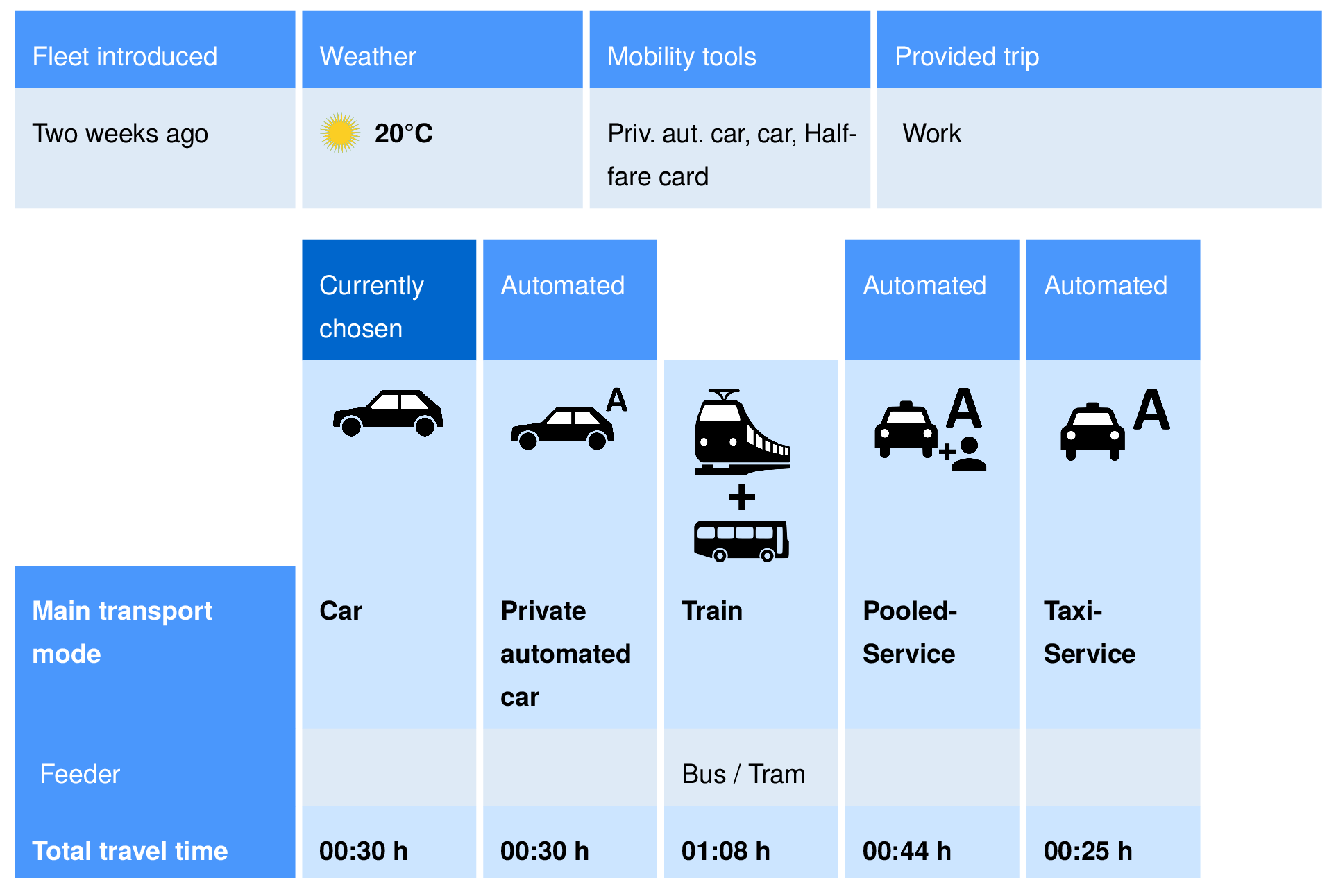
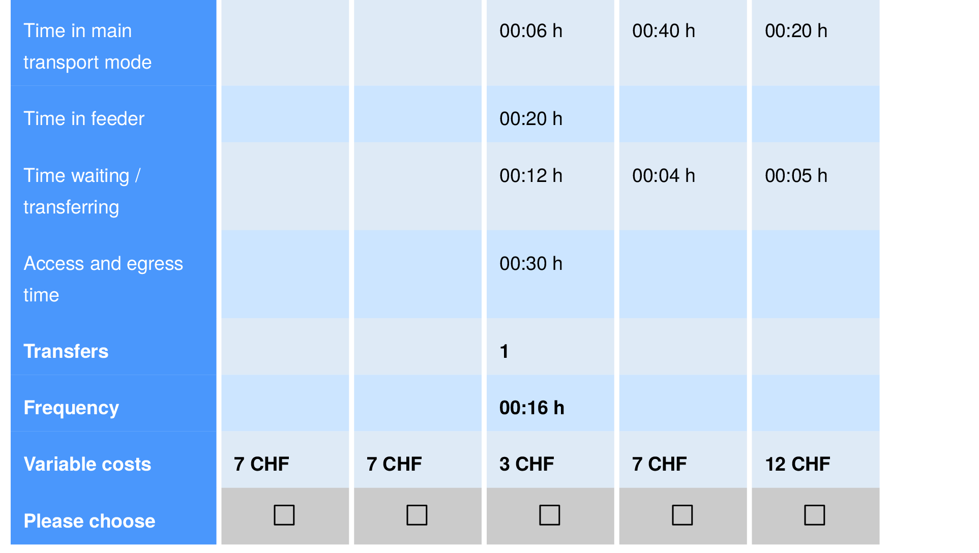
Stated preference survey
MATSim simulation
1
2
3
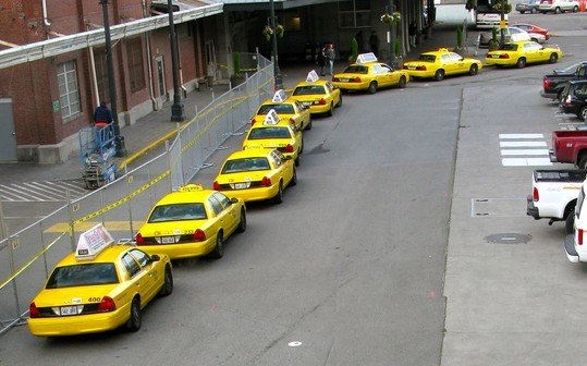
What do we know about automated taxis?
What do we know about automated taxis?

Bösch, P.M., F. Becker, H. Becker and K.W. Axhausen (2018) Cost-based analysis of autonomous mobility services, Transport Policy, 64, 76-91
What do we know about automated taxis?
Felix Becker, Institute for Transport Planning and Systems, ETH Zurich.
VTTS


13 CHF/h
AMoD
Taxi
19 CHF/h
Conventional
Car
12 CHF/h
Public
Transport
AMoD
Car by Adrien Coquet from the Noun Project
Bus by Simon Farkas from the Noun Project
Wait by ibrandify from the Noun Project
VTTS
13 CHF/h
AMoD
Taxi
19 CHF/h
Conventional
Car
12 CHF/h
Public
Transport

21 CHF/h
32 CHF/h
AMoD
Car by Adrien Coquet from the Noun Project
Bus by Simon Farkas from the Noun Project
Wait by ibrandify from the Noun Project
Model structure
Cost calculator
Plan modification
Discrete Mode Choice Extension
Mobility simulation
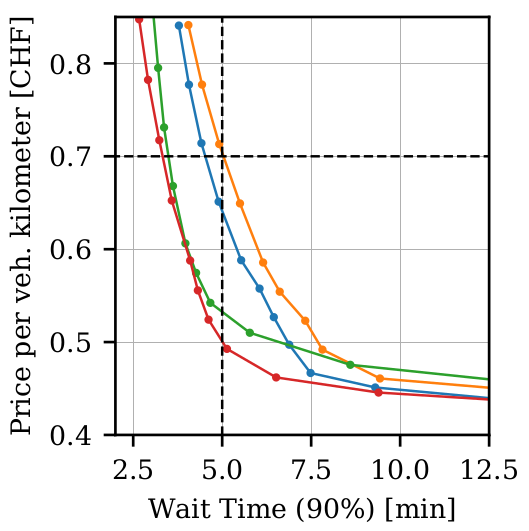
Prediction
Price
Trips
- Utilization
- Empty distance, ...
- Travel times
- Wait times, ...
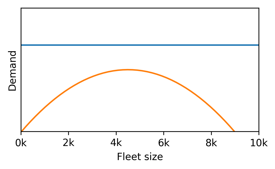
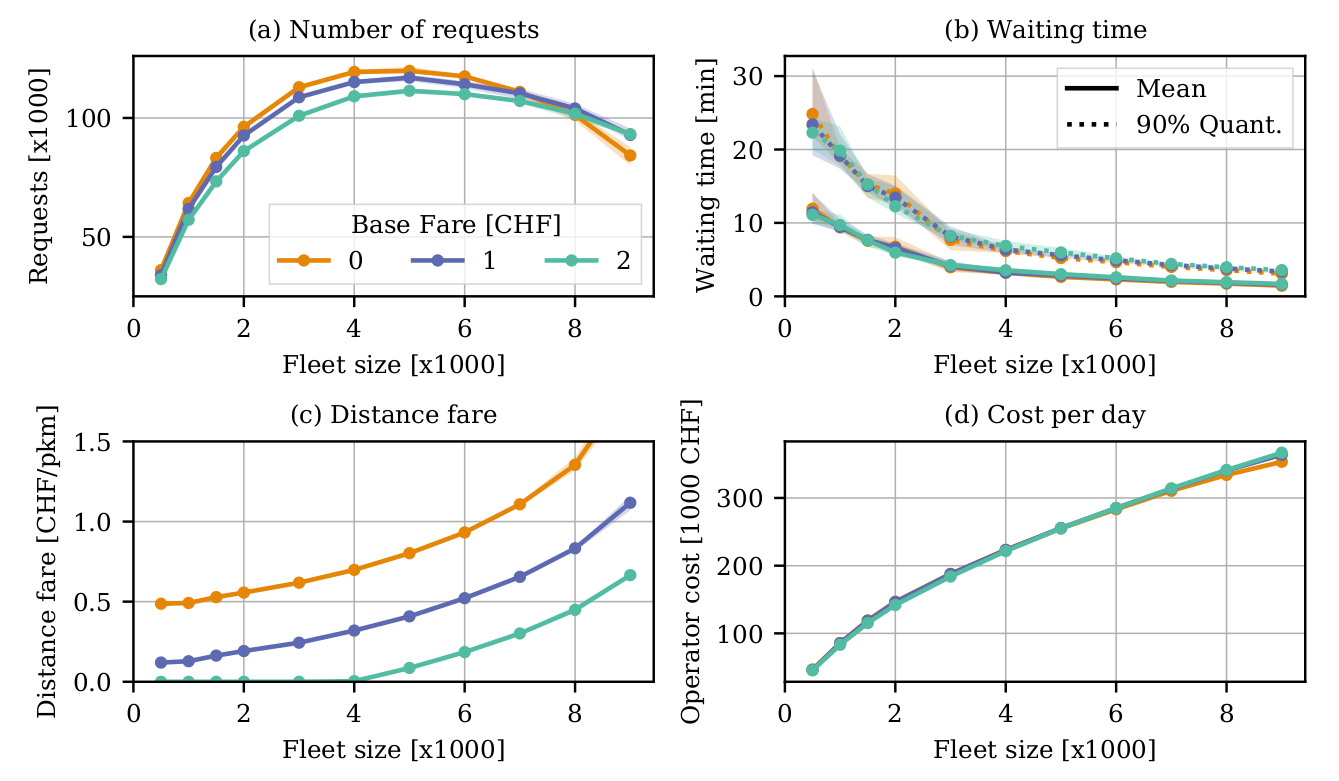
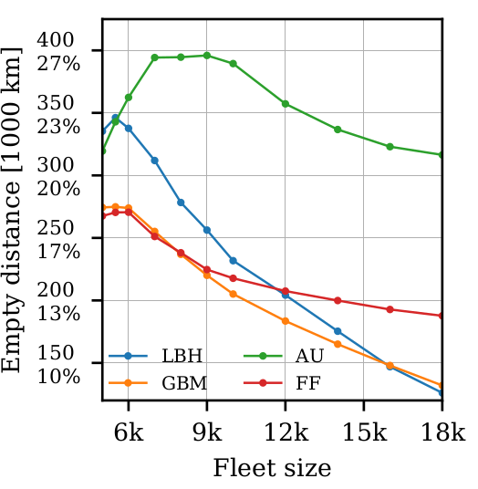
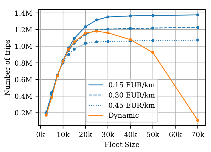
Fleet sizing with dynamic demand
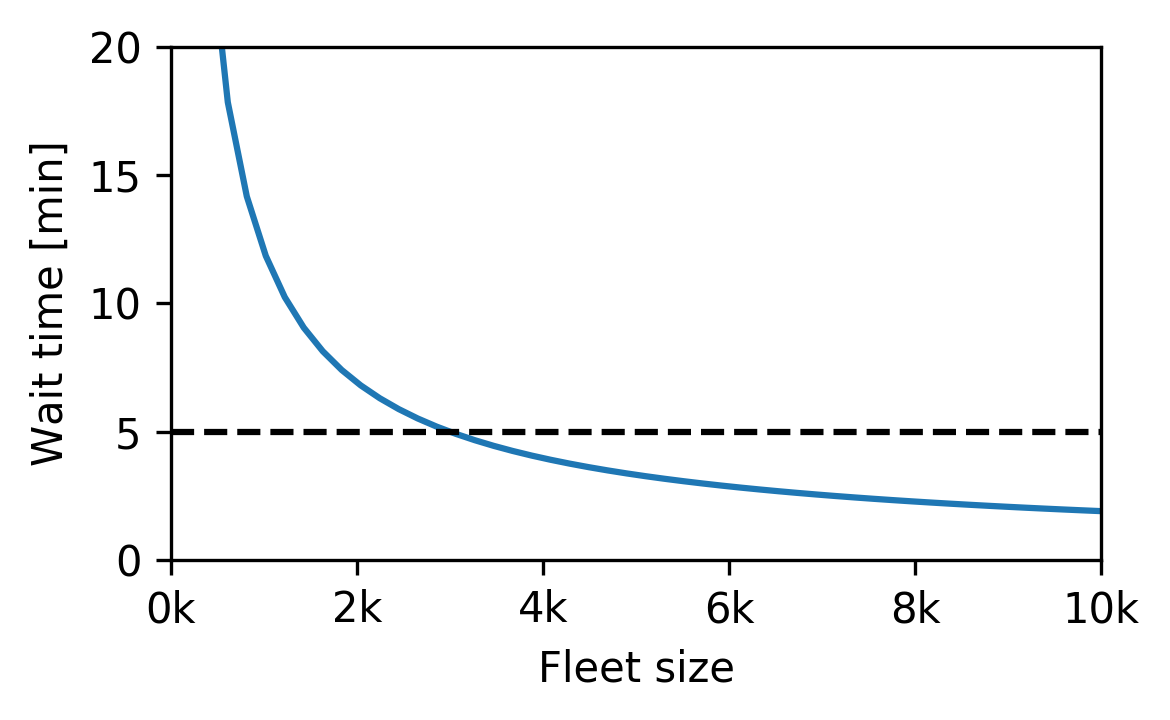
Fleet sizing with dynamic demand
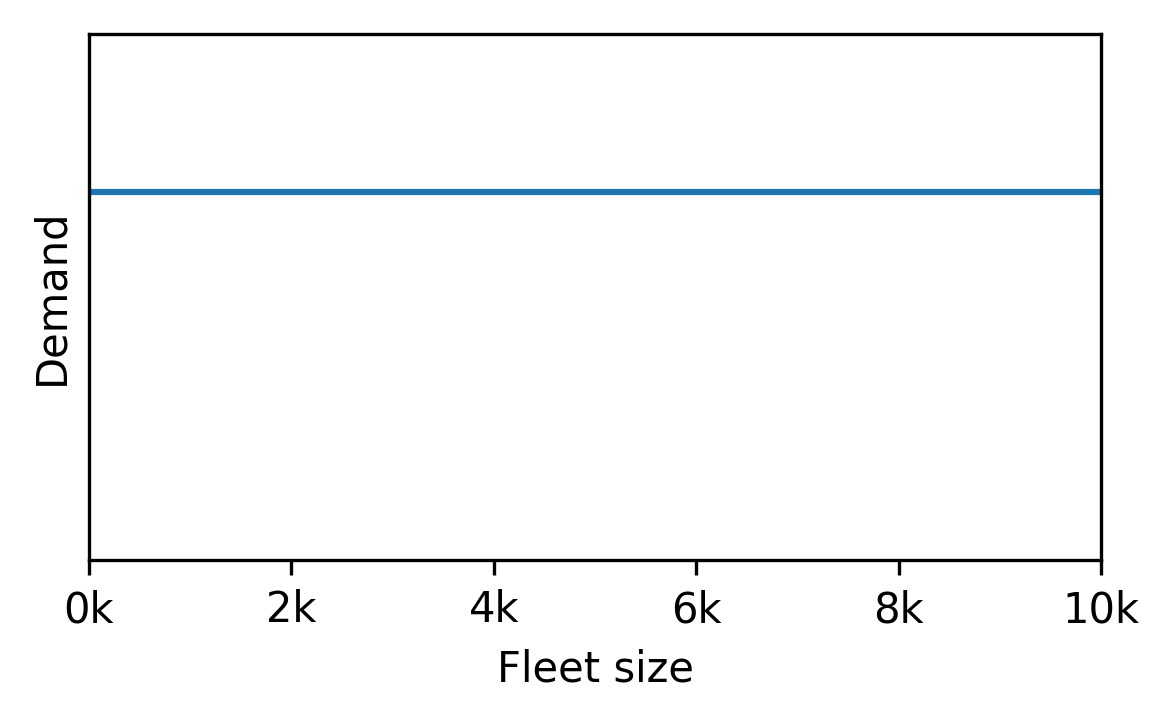
Fleet sizing with dynamic demand
Visualisation
Automated taxi
Pickup
Dropoff
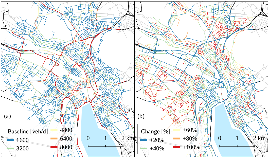
Hörl, S., F. Becker and K.W. Axhausen (2020) Automated Mobility on Demand: A comprehensive simulation study of cost, behaviour and system impact for Zurich
Hörl, S., F. Becker and K.W. Axhausen (2020) Automated Mobility on Demand: A comprehensive simulation study of cost, behaviour and system impact for Zurich
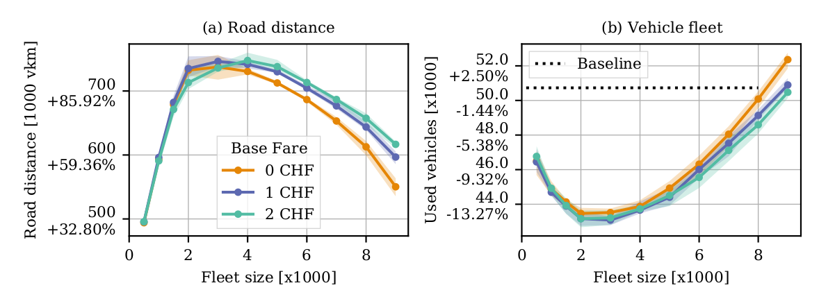
13% reduction in vehicles
100% increase in VKT
Hörl, S., F. Becker and K.W. Axhausen (2020) Automated Mobility on Demand: A comprehensive simulation study of cost, behaviour and system impact for Zurich
100% increase in VKT
Hörl, S., F. Becker and K.W. Axhausen (2020) Automated Mobility on Demand: A comprehensive simulation study of cost, behaviour and system impact for Zurich
Other aspects
Hörl, S., C. Ruch, F. Becker, E. Frazzoli and K.W. Axhausen (2019) Fleet operational policies for automated mobility: a simulation assessment for Zurich, Transportation Research: Part C, 102, 20-32.
Fleet control

Operational constraints
Spatial constraints
Intermodality
Pooling
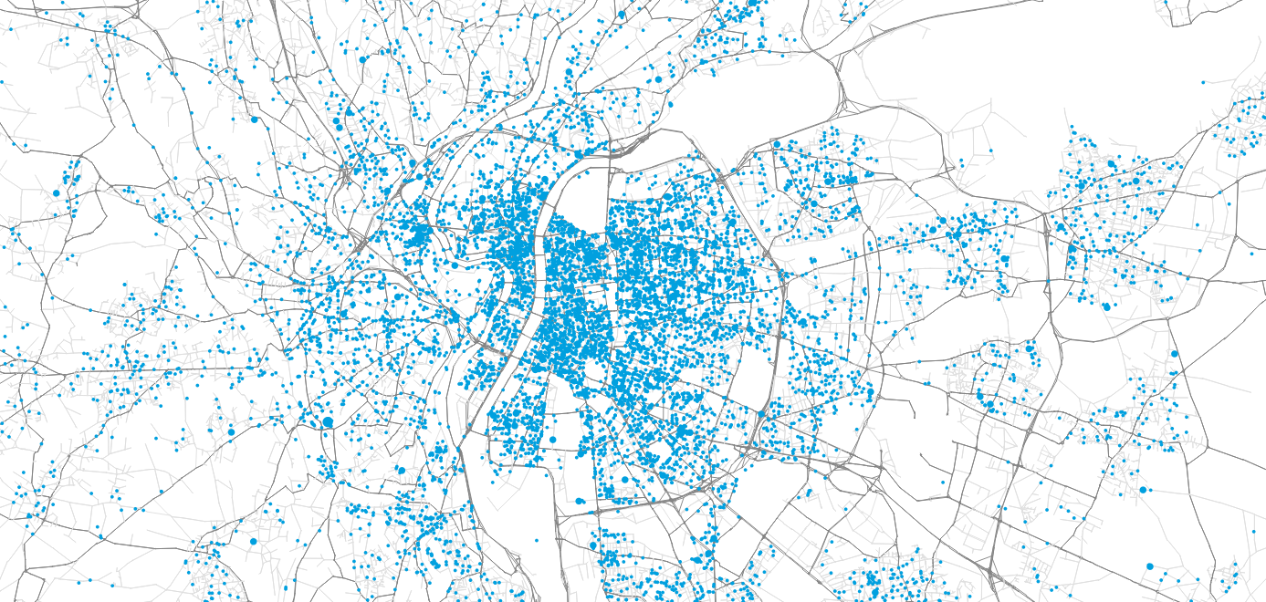
III. Demand data
https://pixabay.com/en/paris-eiffel-tower-night-city-view-3296269/
Synthetic travel demand

Population census (RP)
Population census (RP)
Income data (FiLoSoFi)

Synthetic travel demand
Population census (RP)
Income data (FiLoSoFi)
Commuting data (RP-MOB)
Synthetic travel demand
Population census (RP)
Income data (FiLoSoFi)
Commuting data (RP-MOB)

Household travel survey (EDGT)
0:00 - 8:00
08:30 - 17:00
17:30 - 0:00
0:00 - 9:00
10:00 - 17:30
17:45 - 21:00
22:00 - 0:00
Synthetic travel demand
Population census (RP)
Income data (FiLoSoFi)
Commuting data (RP-MOB)
Household travel survey (EDGT)
Enterprise census (SIRENE)


Address database (BD-TOPO)
Synthetic travel demand
Population census (RP)
Income data (FiLoSoFi)
Commuting data (RP-MOB)
Household travel survey (EDGT)
Enterprise census (SIRENE)
Address database (BD-TOPO)
Person ID
Age
Gender
Home (X,Y)
1
43
male
(65345, ...)
2
24
female
(65345, ...)
3
9
female
(65345, ...)
Synthetic travel demand
Population census (RP)
Income data (FiLoSoFi)
Commuting data (RP-MOB)
Household travel survey (EDGT)
Enterprise census (SIRENE)
Address database (BD-TOPO)
Person ID
Activity
Start
End
Loc.
523
home
08:00
(x,y)
523
work
08:55
18:12
(x,y)
523
shop
19:10
19:25
(x,y)
523
home
19:40
(x,y)
Synthetic travel demand
Population census (RP)
Income data (FiLoSoFi)
Commuting data (RP-MOB)
Household travel survey (EDGT)
Enterprise census (SIRENE)
OpenStreetMap
GTFS (SYTRAL / SNCF)
Address database (BD-TOPO)
Synthetic travel demand
Population census (RP)
Income data (FiLoSoFi)
Commuting data (RP-MOB)
Household travel survey (EDGT)
Enterprise census (SIRENE)
OpenStreetMap
GTFS (SYTRAL / SNCF)
Address database (BD-TOPO)
Synthetic travel demand
Population census (RP)
Income data (FiLoSoFi)
Commuting data (RP-MOB)
National HTS (ENTD)
Enterprise census (SIRENE)
OpenStreetMap
GTFS (SYTRAL / SNCF)
Address database (BD-TOPO)
Synthetic travel demand
EDGT
Population census (RP)
Income data (FiLoSoFi)
Commuting data (RP-MOB)
Enterprise census (SIRENE)
OpenStreetMap
GTFS (SYTRAL / SNCF)
Address database (BD-TOPO)
Synthetic travel demand
Open
Data

Open
Software
+
=
Reproducible research
Integrated testing
National HTS (ENTD)
EDGT
Population census (RP)
Income data (FiLoSoFi)
Commuting data (RP-MOB)
Enterprise census (SIRENE)
OpenStreetMap
GTFS (SYTRAL / SNCF)
Address database (BD-TOPO)
Synthetic travel demand
Open
Data
Open
Software
+
=
Reproducible research
Integrated testing
National HTS (ENTD)
EDGT
Current use cases

Nantes
- Noise modeling
Current use cases
Lille
- Park & ride applications
- Road pricing

Current use cases
Toulouse
- Placement and use of shared offices
Current use cases
Rennes
- Micromobility simulation

Current use cases
Paris / Île-de-France
- Scenario development for sustainable urban transformation
- New mobility services
Mahdi Zargayouna (GRETTIA / Univ. Gustave Eiffel)
Nicolas Coulombel (LVMT / ENPC)
Current use cases

Paris / Île-de-France
- Cycling simulation
Current use cases
Paris / Île-de-France
- Simulation of dynamic mobility services
- Fleet control through reinforcement learning
Current use cases

Lyon (IRT SystemX)
- Low-emission first/last mile logistics
Current use cases
Current use cases
Balac, M., Hörl, S., 2021. Synthetic population for the state of California based on open-data: examples of San Francisco Bay area and San Diego County, in: 100th Annual Meeting of the Transportation Research Board. Washington, D.C., January 2021.
Sallard, A., Balać, M., Hörl, S., 2021. An open data-driven approach for travel demand synthesis: an application to São Paulo. Regional Studies, Regional Science 8, 371–386.
Sao Paulo, San Francisco Bay area, Los Angeles five-county area, Switzerland, Montreal, Quebec City, Jakarta, Casablanca, ...
Emissions in Paris
Grand Paris Express
Automated taxis in Paris
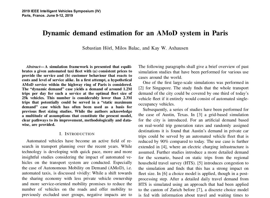
Automated taxis in Paris
IV. Logistics
LEAD Project
Low-emission Adaptive last-mile logistics supporting on-demand economy through Digital Twins
- H2020 Project from 2020 to 2023
- Six living labs with different innovative logistics concepts
- Lyon, The Hague, Madrid, Budapest, Porto, Oslo
- One partner for implementation and one for research each
- Development of a generic modeling library for last-mile logistics scenario simulation and analysis
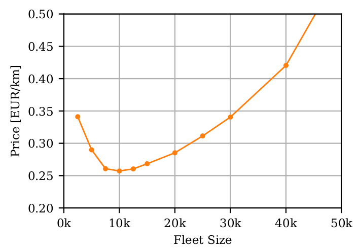
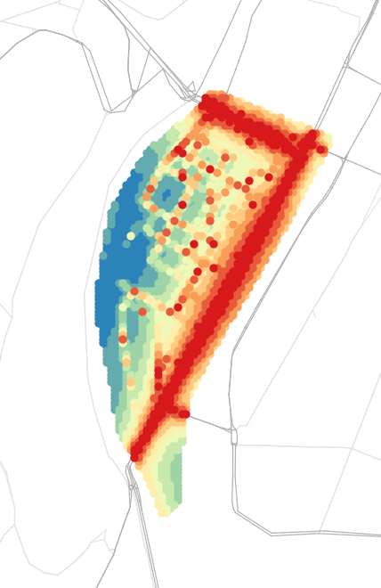
Lyon Living Lab
- Peninsula Confluence between Saône and Rhône
- Interesting use case as there are limited access points
- Implementation of an urban consolidation center (UCC) to collect the flow of goods and organize last-mile distribution
- using cargo-bikes
- using electric robots
- and others
- Analysis and modeling through
- Flow estimation through cameras
- Simulation of future scenarios
- Focus on parcel deliveries due to data availability
Modeling methodology

Agent-based simulation of Lyon
Demand in parcel deliveries
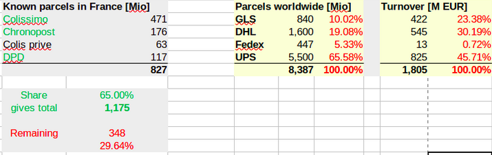
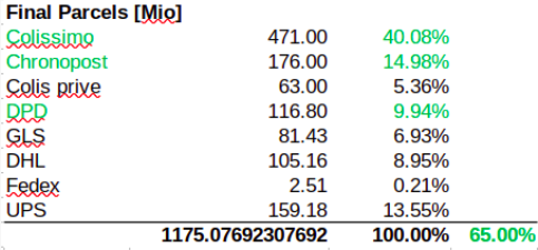
Distribution by operators
KPI Calculation
- Main question: What is the impact on traffic and population of implementing an Urban Consolidation Center in Confluence?
- Focus on B2C parcel deliveries due to data availability
Methodology: Parcel demand
Synthetic population
+
Synthetic population
Out-of-home purchase survey
Achats découplés des ménages
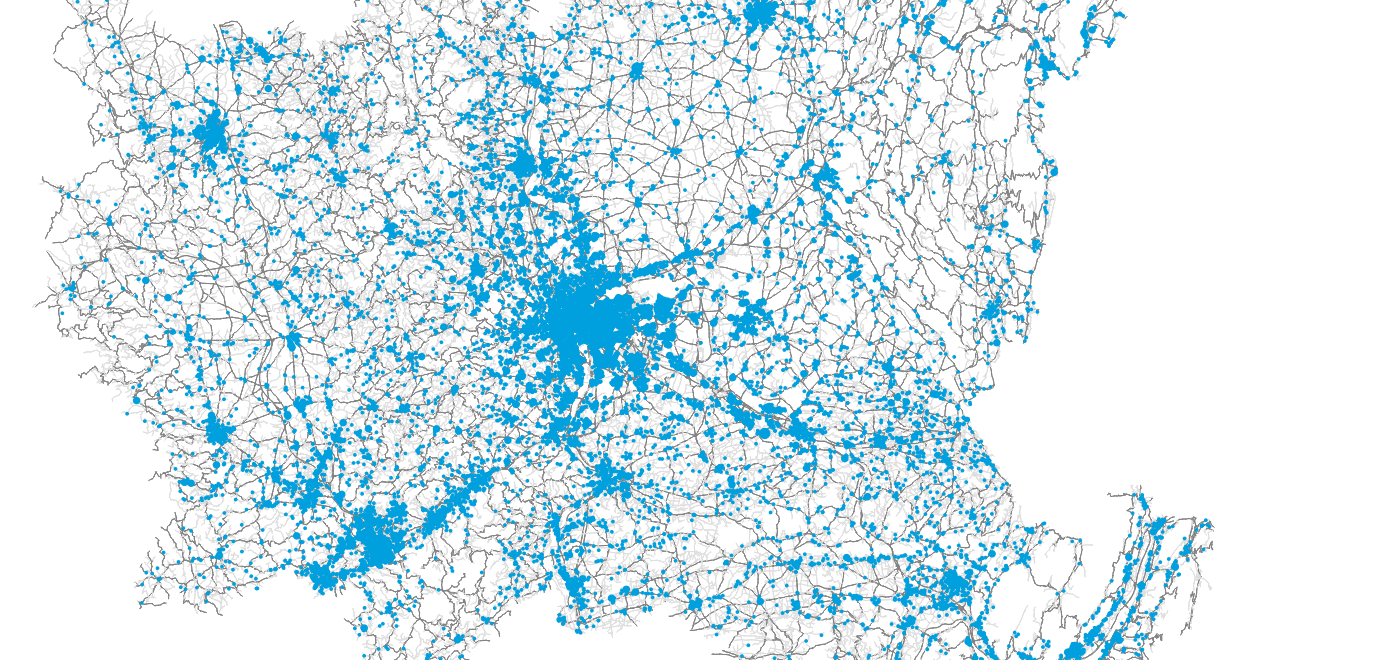
Based on sociodemographic attributes of the households, parcels are generated for the city on an average day.
Gardrat, M., 2019. Méthodologie d’enquête: le découplage de l’achat et de la récupération des marchandises par les ménages. LAET, Lyon, France.
Methodology: Parcel demand
Synthetic population
+
Synthetic population
Out-of-home purchase survey
Achats découplés des ménages
Based on sociodemographic attributes of the households, parcels are generated for the city on an average day.
Gardrat, M., 2019. Méthodologie d’enquête: le découplage de l’achat et de la récupération des marchandises par les ménages. LAET, Lyon, France.
Methodology: Parcel demand
Synthetic population
Gardrat, M., 2019. Méthodologie d’enquête: le découplage de l’achat et de la récupération des marchandises par les ménages. LAET, Lyon, France.
+
Synthetic population
Out-of-home purchase survey
Achats découplés des ménages
Based on sociodemographic attributes of the households, parcels are generated for the city on an average day.
Iterative proportional fitting (IFP)
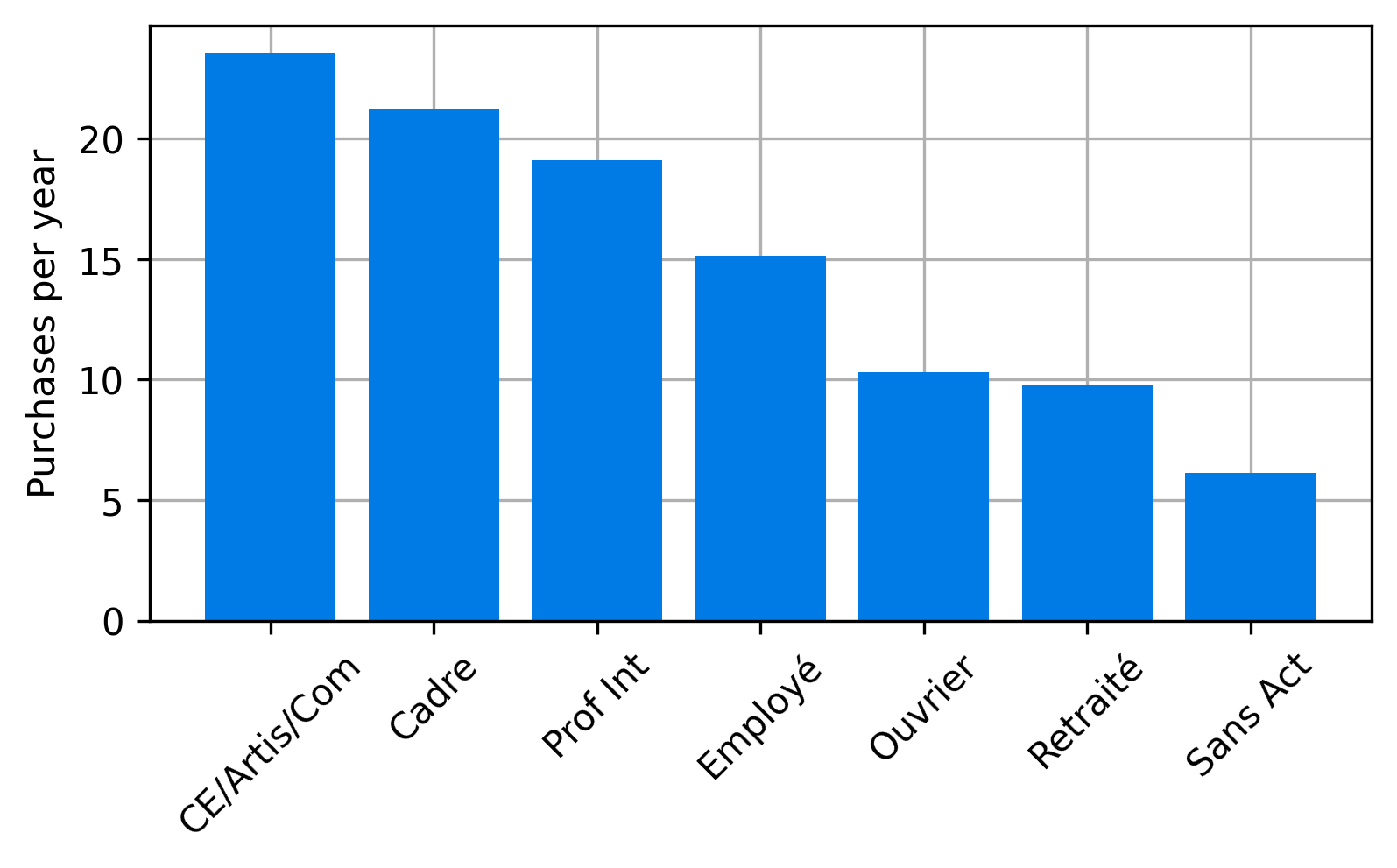
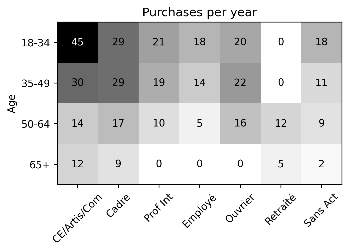
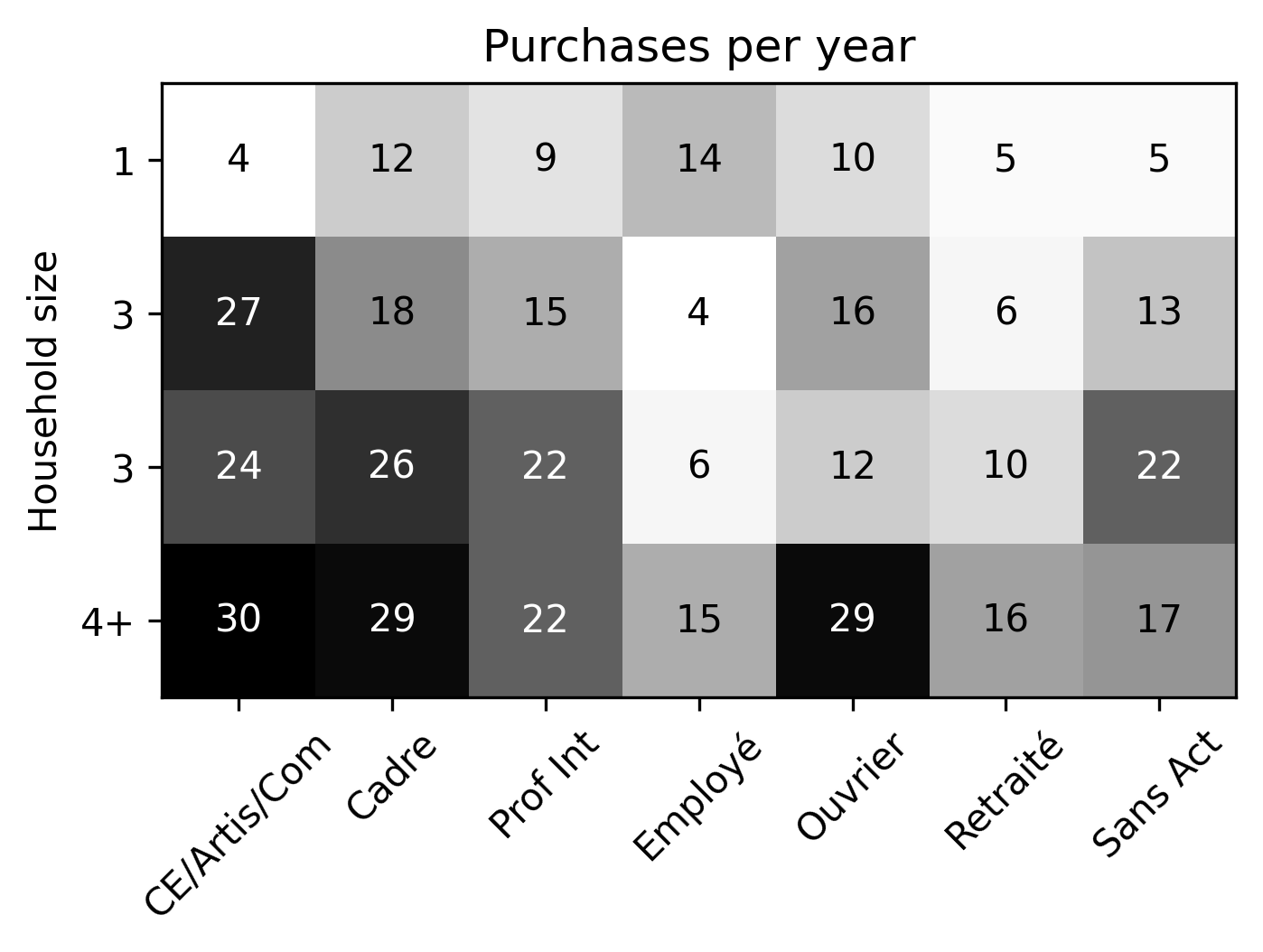
- Based on synthetic population, find average number of purchases delivered to a household defined by socioprofesional class, age of the reference person and household size per day.
\mu_{a,h,s} = d_{s} \cdot \frac{w_{a,h,s}}{365}
Methodology: Parcel demand
Synthetic population
Gardrat, M., 2019. Méthodologie d’enquête: le découplage de l’achat et de la récupération des marchandises par les ménages. LAET, Lyon, France.
+
Synthetic population
Out-of-home purchase survey
Achats découplés des ménages
Based on sociodemographic attributes of the households, parcels are generated for the city on an average day.
Maximum entropy approach
- We now the average number of parcels, but we do not now the distribution of the number of parcels for a household on an average day.
- We know it must be non-negative, and we know the mean.
- Without additional data, we assume maximum entropy distribution, which is Poisson in this case.
F(N \leq n) = \text{Pois}(\mu)
Methodology: Parcel demand
Synthetic population
Gardrat, M., 2019. Méthodologie d’enquête: le découplage de l’achat et de la récupération des marchandises par les ménages. LAET, Lyon, France.
+
Synthetic population
Out-of-home purchase survey
Achats découplés des ménages
Based on sociodemographic attributes of the households, parcels are generated for the city on an average day.
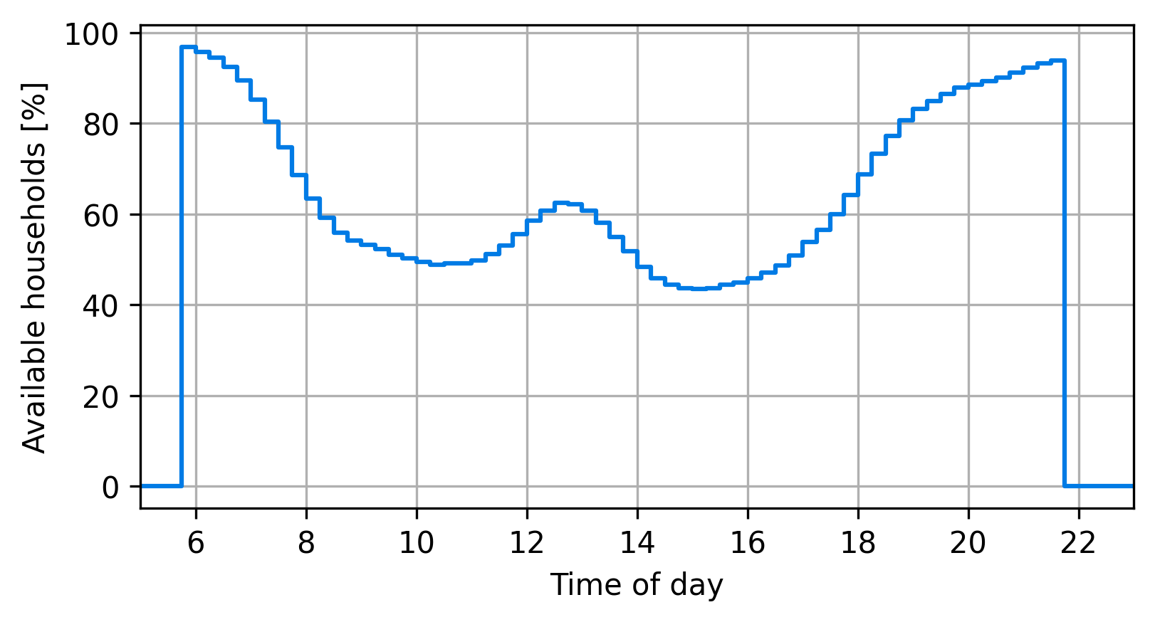
Presence of household members
Methodology: Route optimization
Using a heursitic routing solver, an optimal distribution scheme per distribution center is obtained to arrive at a lower bound estimate for the distance covered for the deliveries.

JSprit
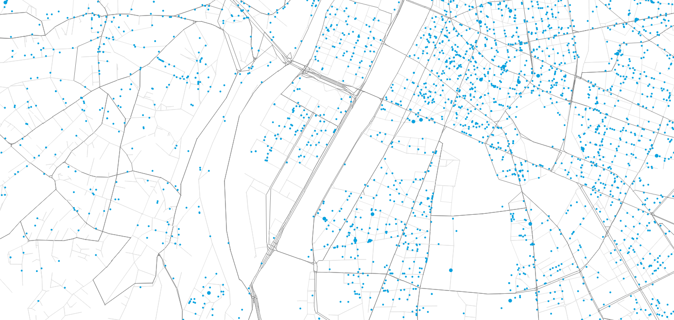
First case study
Hörl, S. and J. Puchinger (2021) From synthetic population to parcel demand: Modeling pipeline and case study for last-mile deliveries in Lyon, Working paper.
Solve VRP-TW based on generated parcels and household presence
JSprit
First case study
Hörl, S. and J. Puchinger (2021) From synthetic population to parcel demand: Modeling pipeline and case study for last-mile deliveries in Lyon, Working paper.
Solve VRP-TW based on generated parcels and household presence
JSprit

Scaling up: City-wide baseline
Using shares of customer preference, parcels are assigned to operators and the closest distribution centers.
SIRENE: Delivery centers
Scaling up: City-wide baseline
Using shares of customer preference, parcels are assigned to operators and the closest distribution centers.
SIRENE: Delivery centers
Scaling up: City-wide baseline
Using shares of customer preference, parcels are assigned to operators and the closest distribution centers.
SIRENE: Delivery centers
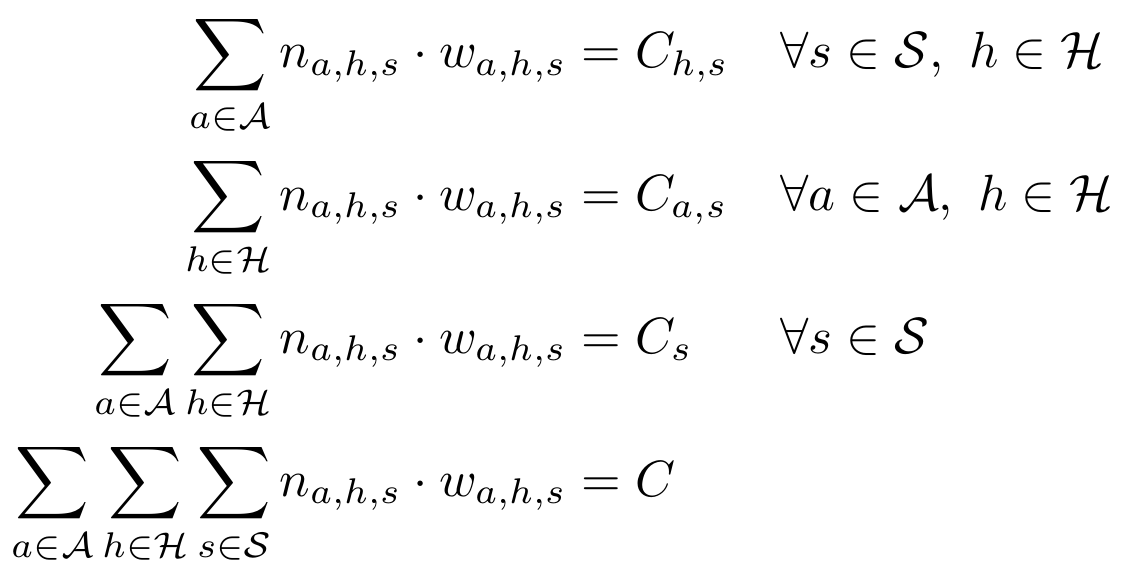
Methodology: Supply side
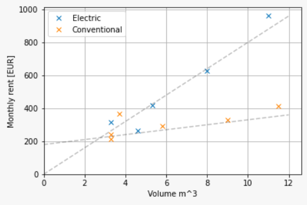
Vehicle routing and fleet composition problem
- Minimize total cost of delivering all parcels for each center
- Distance cost influenced by fuel / electricity cost
- Fixed cost (per day) influenced by salaries and vehicle cost
- Derive
- Distances driven and related emissions
- Fleet composition for each center

Novel approximation method
Visualisation platform
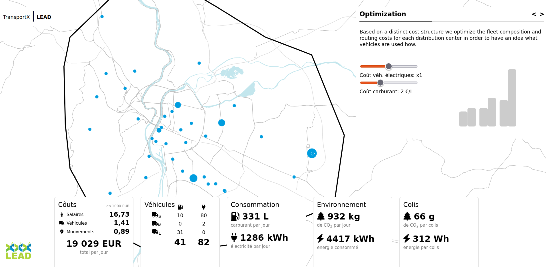
UCC platform
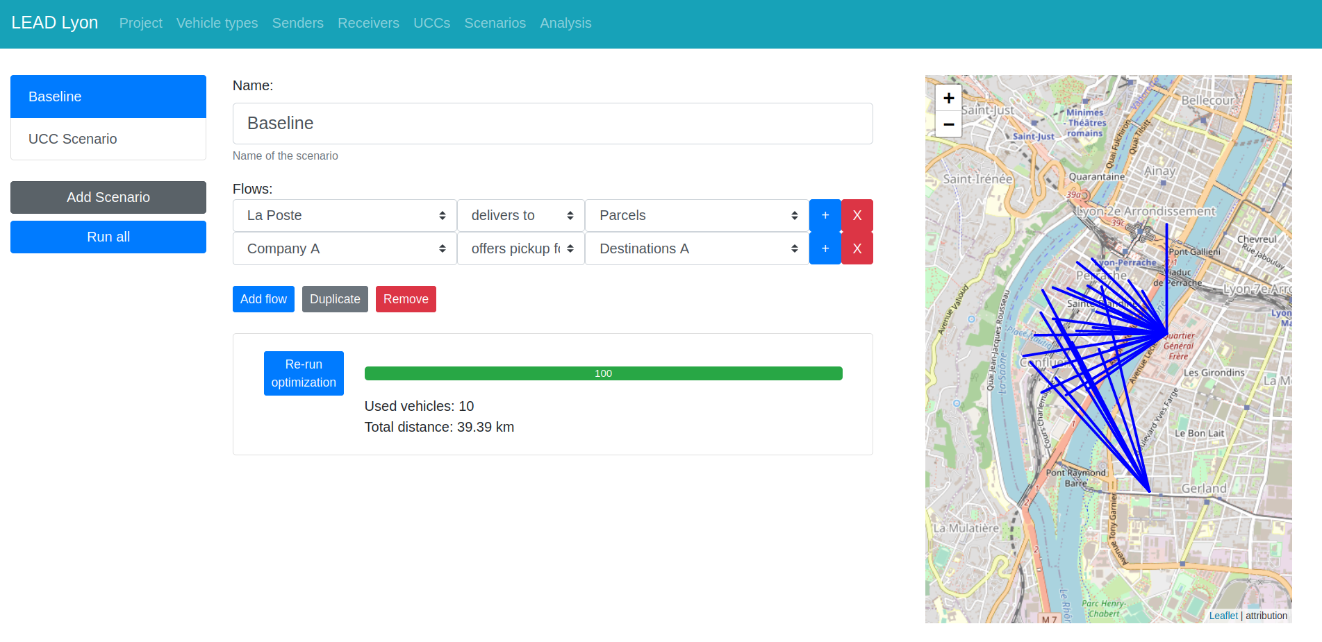
Timeline
- Lectures
- 10/01 8h30: Examples of large-scale models in transportation
- 10/01 10h45: Modeling methods I
- 13/01 14h00: Modeling methods II
- 13/01 16h45: Introduction to the student project
- Project work
- 27/01 14h00 + 16h45: Intermediate results
- 09/02 14h00 + 16h45: Exchange with other groups
- 23/02 14h00 + 16h45: Final presentation
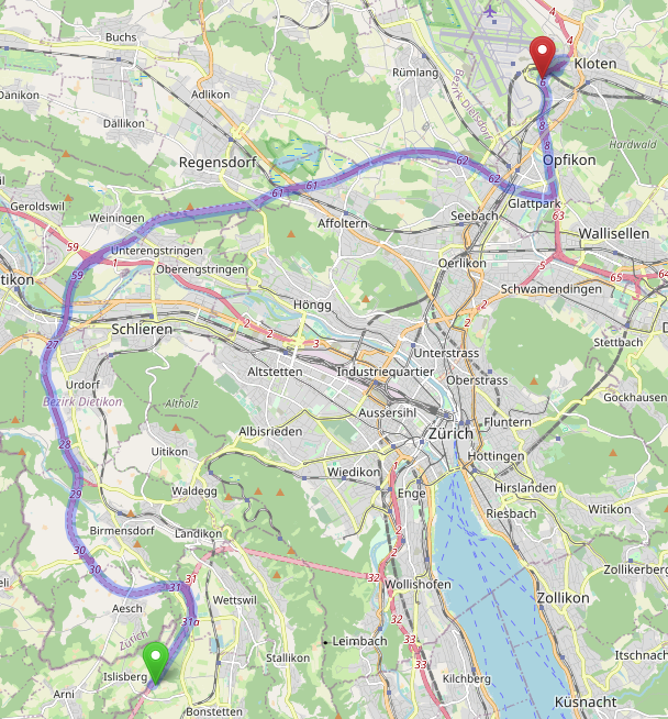
Transport planning: Overview
- Goals
- Cost-benefit analysis
- Assessment of alternatives
- Prediction
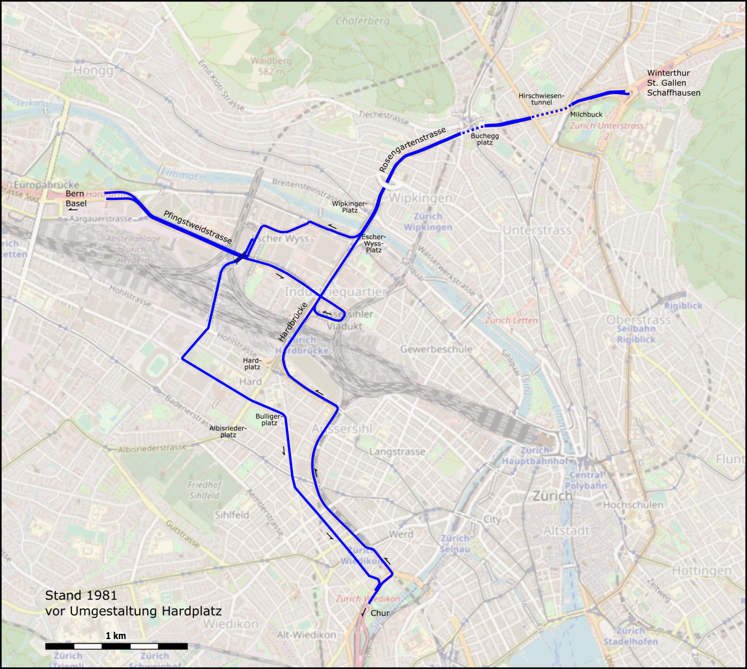
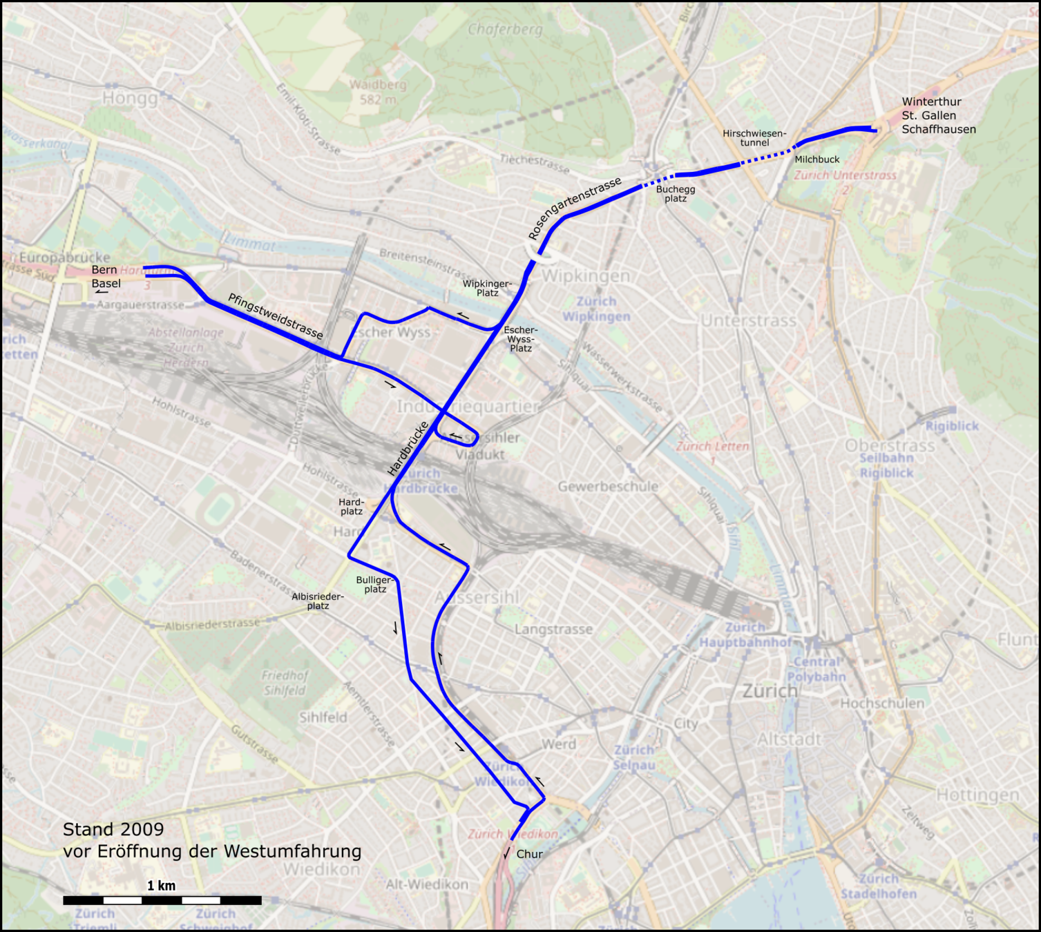
Sources: https://de.wikipedia.org/wiki/Westtangente_Z%C3%BCrich, openstreetmap.org
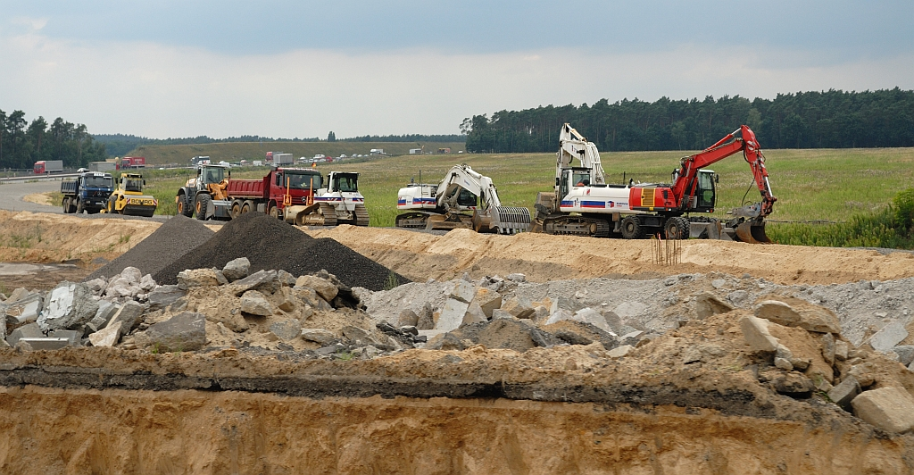
Transport planning: Overview
- Goals
- Cost-benefit analysis
- Assessment of alternatives
- Prediction
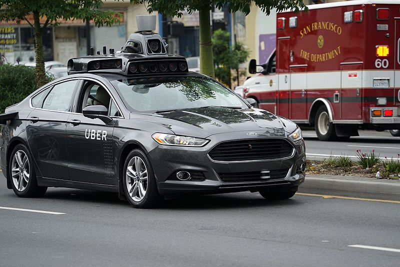
- Use cases
- Traditionally: Infrastructure
- Today: Increasingly digital technology
Sources:
https://en.wikipedia.org/wiki/File:Highway_8_widening.png
https://commons.wikimedia.org/wiki/File:Self_driving_Uber_prototype_in_San_Francisco.jpg
Transport planning: Overview
- Traditional approaches
- High aggregation
- Movements are flows
- Locations are zones
- Specific times of the day
- Today's approaches
- Individual entities
- Movements are detailed in time and space
- Whole daily analysis possible
Four-step models
Activity-based models
Four-step model: Overview
Generation
Distribution
Mode choice
Assignment
- Four steps making use of different data sources
- From static to more dynamic mobility decisions
- Multiple possible feedback loops (most common example here)
Four-step model: Overview
Generation
Distribution
Mode choice
Assignment
- Where do trips appear?
- What is the destination of the trips?
- What transport mode is used?
- What congestion is caused?
Four-step model: Overview
Generation
Distribution
Mode choice
Assignment
Travel demand
Travel supply
- Characterizes the need for mobility in the population for economic activity, leisure, ...
- Means that allow for mobility
- Road infrastructure, rail network, ...
Four-step model: Overview
Generation
Distribution
Mode choice
Assignment
Travel demand
Travel supply
- Characterizes the need for mobility in the population for economic activity, leisure, ...
- Means that allow for mobility
- Road infrastructure, rail network, ...
Equilibrium
- Given limited capacity,
how is the system used?
Four-step model: Trip generation
-
Goal: Define statistically where trips starts, i.e. where they are "generated" or produced
- Focus on peak hours in 4S, e.g. morning peak and focus on commuting activity
- Either making use of direct data (e.g. from surveys) or based on population data, land use information, ...
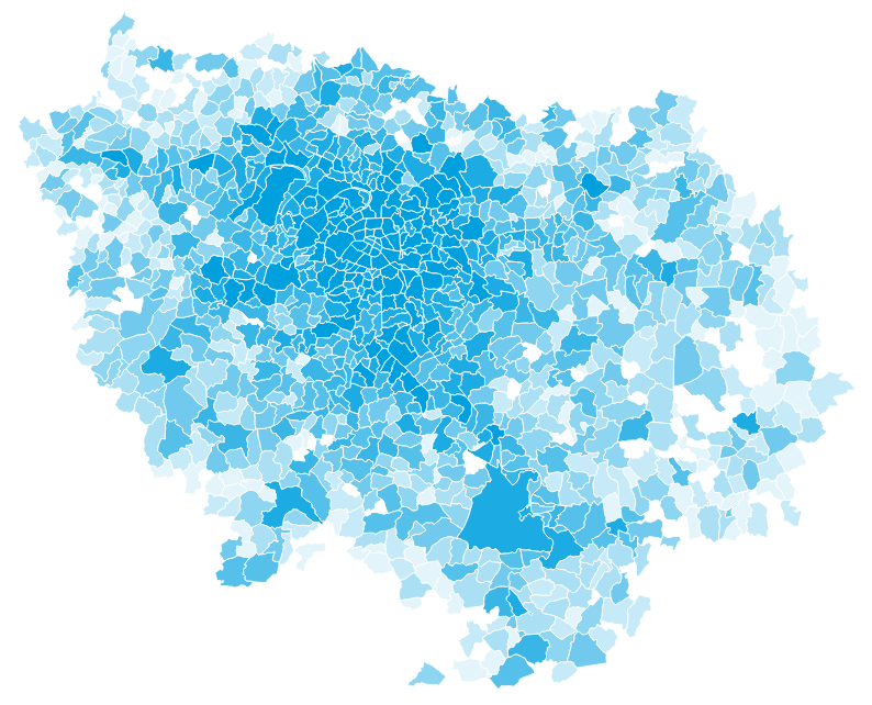
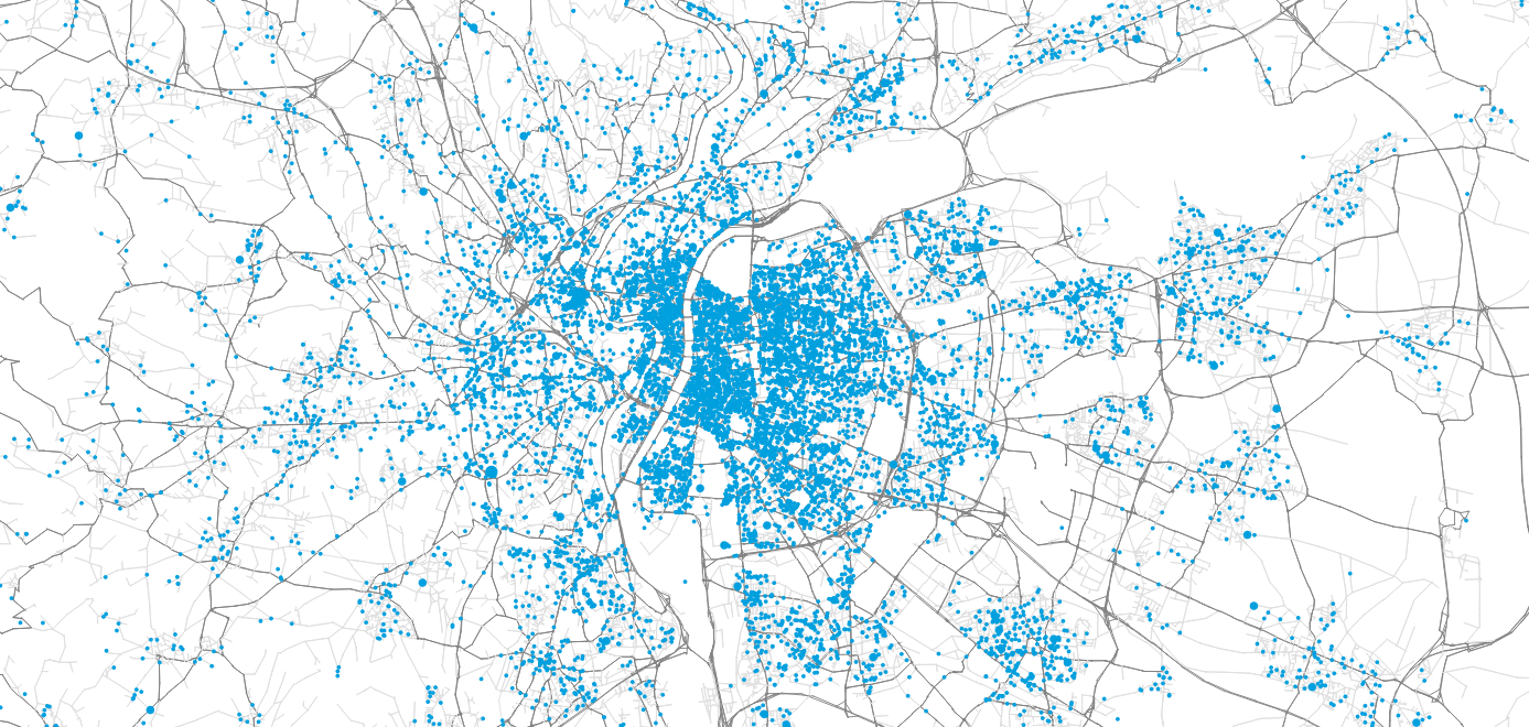
Number of inabitants in Île-de-France
Four-step model: Trip generation
- May be per homogeneous user group, e.g.
- Single-person households
- Multi-persons households
without children - Multi-person households
with children -
Households with retired persons
- Possible to use statistical models
O_{s,g} = f(X_s)
Generated trips
in zone s in group g
Trip generation model
Model inputs
Four-step model: Trip generation
- Example: Linear model based on socioprofessional category (CS):
- Employee
- Worker
- Retired
-
...
- Do we have reference number of trips for some of the zones? Then we can create a model from this formula! Example: Ordinary Least Squares (OLS)
f(X) = \sum_{CS} \lambda_{CS} \cdot x_{CS}
Model parameters (linear factors)
Census data (inhabitants)
\text{min}_\Lambda \sum_s (f(X_s|\Lambda) - \hat O_s)^2
Reference data
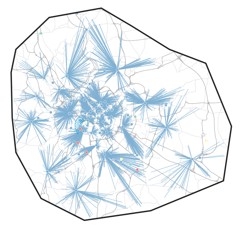
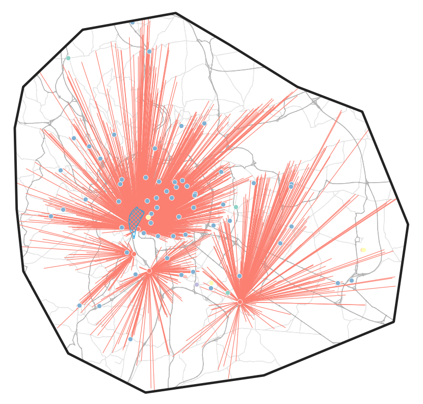
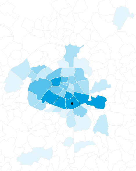
Four-step model: Trip distribution
- Goal: Given the produced trips with their origin zone, define where they end = distribute the trips over a set of potential destination
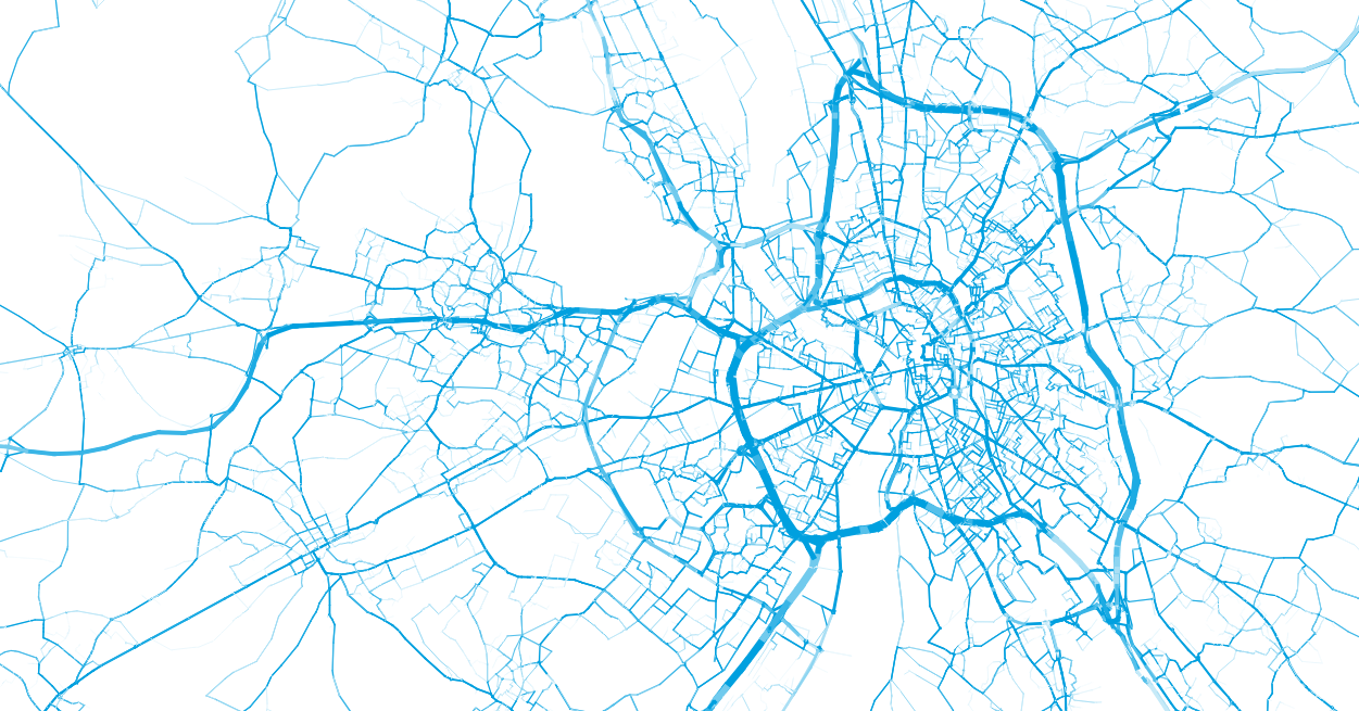
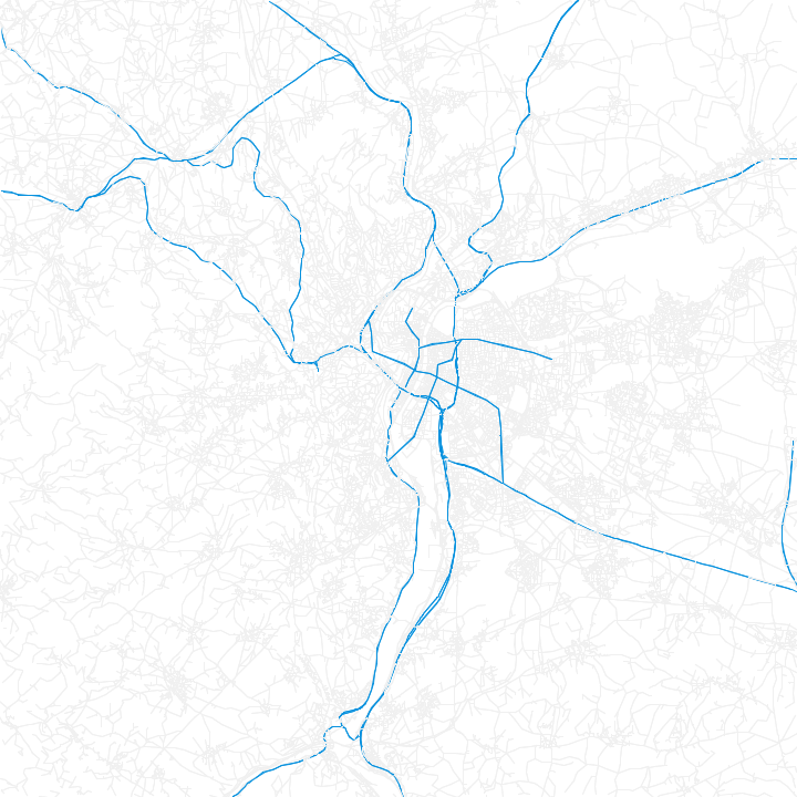
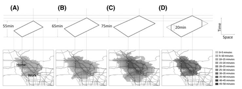
Number of daily commutes arriving from 13th arrondissement
Four-step model: Trip distribution
- Based on trip generation, we want to predict the number of trips going from zone s to zone t
- Various ways to model flows between zones
- Gravity model
- Discrete choice model
-
Maximum entropy
- Can be formulated per group g.
F_{s,t} = f(X_s, X_t)
Flow between s and t
Model
| O1 | ... | ... | On | |
|---|---|---|---|---|
| D1 | ||||
| ... | Fst | |||
| ... | ||||
| Dn |
O_s
D_t
Four-step model: Trip distribution
- Growth factor approach
- Useful if information on existing flows is available for many relations and we want to obtain an explicative model
- Useful if information on existing flows is available for many relations and we want to obtain an explicative model
- Constrained approach
- We have little flow information, but know about the total in each zone (e.g. population and workplaces)
F_{s,t} = \lambda_{s,t} \cdot O_t
\lambda_{s,t} = f(X_s, X_t)
Trip generation
Growth factor modeled through zone attributes
D_t = \sum_s F_{s,t}
O_s = \sum_t F_{s,t}
F_{s,t} = f(X_s, X_t)
Require
with
Four-step model: Trip distribution
- Common approach: Gravity model
F_{s,t} = f(X_s, X_t) = \rho \cdot P_s \cdot A_t \cdot R_{s,t}
P_s = P(X_s)
A_t = A(X_t)
Production model, e.g. P = Population or Population Density
Attraction model, e.g. A = Workplaces or Workplace Density
R_{s,t} = A(X_s, X_t)
Resistance model, e.g. based on travel time or distance (also called impedance)
R_{s,t} = exp( -\beta \cdot \text{Distance}(s,t) )
Four-step model: Trip distribution
F_{s,t} = f(X_s, X_t) = \rho \cdot P_s \cdot A_t \cdot R_{s,t}
O_s = \sum_t F_{s,t}
O_s = \sum_t F_{s,t}
- Common approach: Gravity model
-
If we know F, we can calibrate all models, e.g. using OLS ...
- ... but we may better know required origins, i.e.
Four-step model: Trip distribution
F_{s,t} = f(X_s, X_t) = \rho \cdot P_s \cdot A_t \cdot R_{s,t}
O_s = \sum_t F_{s,t}
O_s = \sum_t F_{s,t} = \rho \cdot P_s \cdot \sum_t A_t \cdot R_{s,t}
- Common approach: Gravity model
-
If we know F, we can calibrate all models, e.g. using OLS ...
- ... but we may better know required origins, i.e.
Four-step model: Trip distribution
- Common approach: Gravity model
-
If we know F, we can calibrate all models, e.g. using OLS ...
-
... but we may better know required origins, i.e.
F_{s,t} = f(X_s, X_t) = \rho \cdot P_s \cdot A_t \cdot R_{s,t}
O_s = \sum_t F_{s,t}
O_s = \sum_t F_{s,t}
P_s = \frac{O_s}{\rho \sum_t A_t R_{s,t}}
Four-step model: Trip distribution
-
... which can be inserted into the model ...
-
... leading to
with
- If R is given or estimated independently (usually the case), the flows F are determined!
F_{s,t} = f(X_s, X_t) = \rho \cdot P_s \cdot A_t \cdot R_{s,t}
\alpha_s = \frac{1}{\sum_t A_t R_{s,t}}
F_{s,t} = f(X_s, X_t) = \alpha_s \cdot A_t \cdot R_{s,t} \cdot O_s
P_s = \frac{O_s}{\rho \sum_t A_t R_{s,t}}
Four-step model: Trip distribution
-
Including both origin and destination constraints gives
with
F_{s,t} = f(X_s, X_t) = \alpha_s \cdot \beta_t \cdot O_s \cdot D_t \cdot R_{s,t}
P_s = \frac{O_s}{\rho \sum_t A_t R_{s,t}}
\alpha_s = \frac{1}{\sum_t A_t R_{s,t}}
\beta_t = \frac{1}{\sum_s P_s R_{s,t}}
A_t = \frac{D_t}{\rho \sum_s P_s R_{s,t}}
- By construction, the origin and destination counts are replicated when iteratively solving
Timeline
- Lectures
- 10/01 8h30: Examples of large-scale models in transportation
- 10/01 10h45: Modeling methods I
- 13/01 14h00: Modeling methods II
- 13/01 16h45: Introduction to the student project
- Project work
- 27/01 14h00 + 16h45: Intermediate results
- 09/02 14h00 + 16h45: Exchange with other groups
- 23/02 14h00 + 16h45: Final presentation
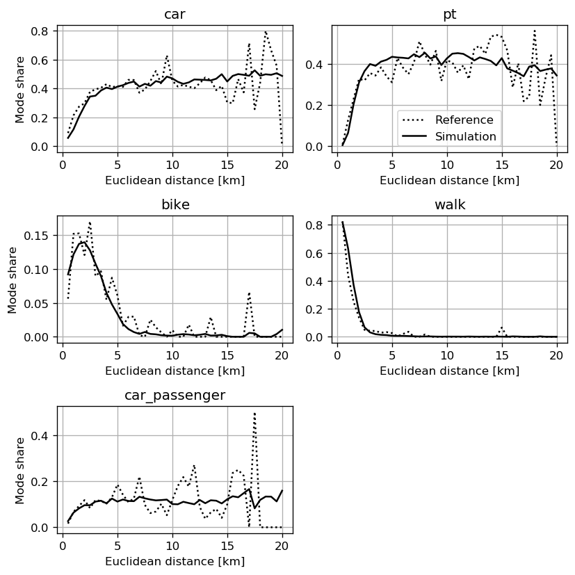
Four-step model: Mode choice
-
Goal: Given the infrastructure and the generated OD trips, which mode of transport should be used for them.
- Expressed as mode share: How many percent of the trips on a OD relation are performed with mode m?
P[m]
m \in \{ car, pt, ... \}
\sum_m P[m] = 1
P[m] \geq 0
Utility maximization
-
Utility maximization is important concept in transport planning: Given a set of choices (modes, destinations, ...) we can assign a utility v to each alternative k.
- We assume rational decision makers that always want to choose the alternative with the highest utility.
- Homo oeconomicus
v_k = \beta^T X
k^* = \text{arg max}_k \{ v_1, ..., v_k, ... v_K \}
Utility maximization
- Example: Choice between two public transport connections
v_k = \beta_\text{travelTime} \cdot x_{k, \text{travelTime}} + \beta_\text{interchanges} \cdot x_{k, \text{interchanges}}
Connection A
x_{A, \text{travelTime}} = 20\ \text{min}
Connection B
x_{B, \text{travelTime}} = 30\ \text{min}
x_{B, \text{interchanges}} = 0
x_{A, \text{interchanges}} = 1
-0.6
-1.0
-0.6 * 20 - 1.0 * 1 = -13
-0.6 * 30 - 1.0 * 0 = -19
Connection A is better alternative.
Utility maximization
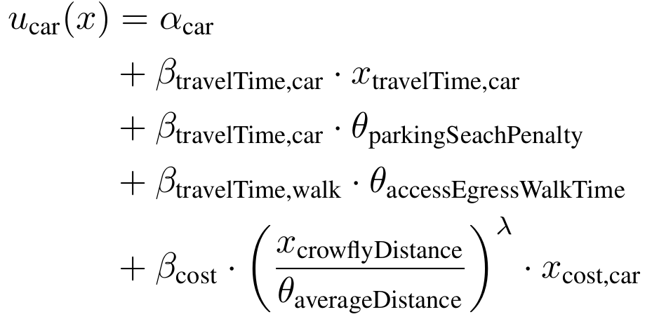
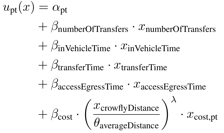
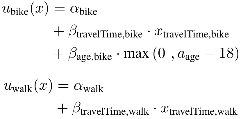
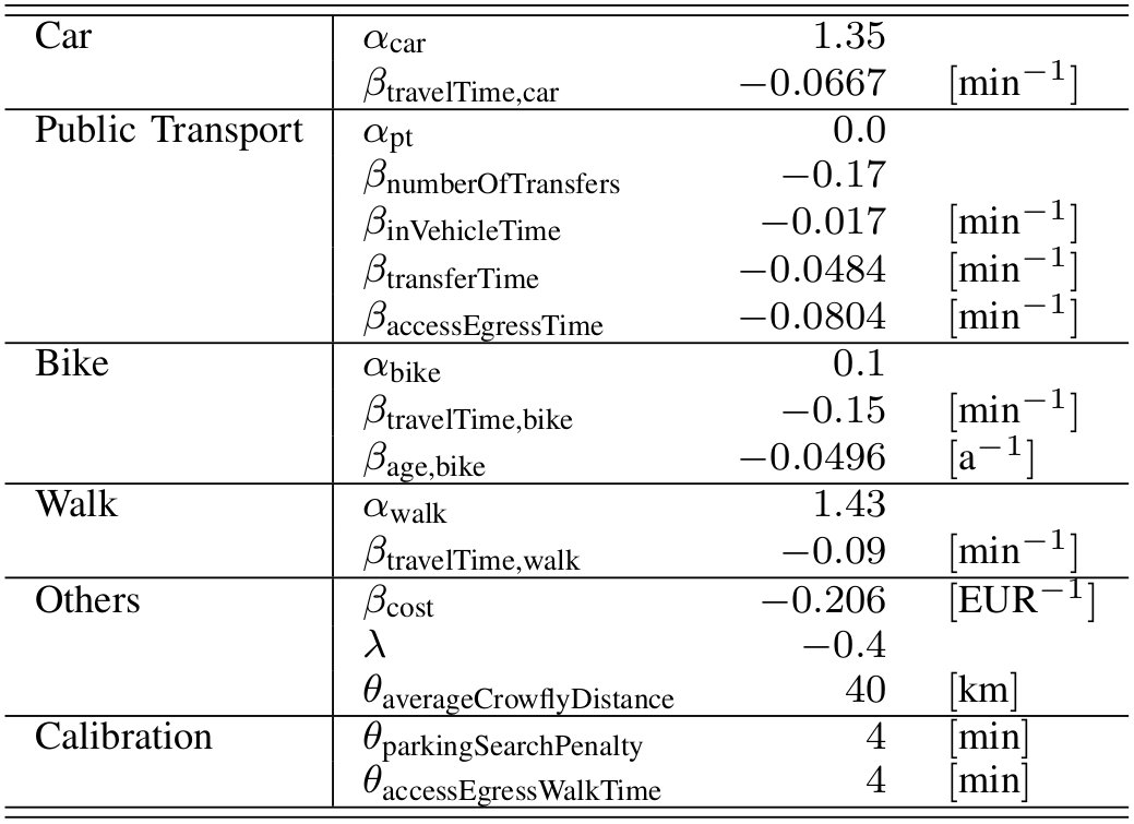
- Example: Mode choice model
Random Utility Models
- How to estimate such models?
- Assume K alternatives and N observed choices y described by index i.
- We want to find the set of parameters such that all choices i are replicated correctly:
v_k(X_i) = \beta^T \cdot X_k
y_i \in \{ 1, ..., K \}
\beta
y_i = \text{arg max}_k \{ v_k(X_i|\beta) \} \ \
\forall i
Find such that
Random Utility Models
- Not easily possible: We cannot model reality sufficiently well, people have own tastes.
- Hence, we introduce an error term.
- This leads to a random utility maximization (RUM) model
u_{k,i} = v_{k,i} + \sigma \epsilon_{k,i}
E[\epsilon_{k,i}] = 0
\sigma \geq 0
k^*_i = \text{arg max}_k \{ u_{k,i} \}
k^*_i = \{ k \ | \ (u_{k,i} \geq u_{1,i}) \land \ (u_{k,i} \geq u_{2,i}) \land ... \}
Random Utility Models
- McFadden has shown in the seventies that if error follows Extreme Value distribution ...
- ... there is a closed form expression for the choice probability:
- Two alternatives k:
Binomial logit model
- Multiple alternatives k:
Multinomial logit model
u_k = v_k + \sigma \epsilon_k
\epsilon_{k,i} \sim \text{EV}
P[k] = \frac{\exp(\sigma^{-1} v_k)}{\sum_{k'}\exp(\sigma^{-1} v_{k'})}
Random Utility Models
- Coming back to estimation:
- Under multinomial logit assumption, we can write a (log-)likelihood function ...
- ... which is proven convex and can be maximized using any optimization method!
P[k] = \frac{\exp(\sigma^{-1} v_k)}{\sum_{k'}\exp(\sigma^{-1} v_{k'})}
v_k(X_i) = \beta^T \cdot X_k
y_i \in \{ 1, ..., K \}
\mathcal{L}(\beta) = \prod_i P[y_i|X_i,\beta]
l(\beta) = \sum_i \log P[y_i|X_i,\beta]
\beta^* = \text{arg max}_{\beta} \sum_i \log P[y_i|X_i,\beta]
Random Utility Models
- Multinomial logit is commonly used and part of larger class of discrete choice models.
- Can also be used in distribution step.
- Last step of 4S model
- What are resulting flows on the roads?
- What are the resulting travel times?
Four-step model: Assignment
- Again, based on rational decision maker
- Game theoretic perspective: Travellers compete about using the roads, each maximizing the utility they gain
- Many ways of solving assignment problem
Four-step model: Assignment
- Example: Two routes
- Travellers on Route A:
- Travellers on Route B:
- Total travellers from S to E:
- Travel time route A (normal road):
- Travel time route B (highway):
- Wardrop principle: Travellers tend to minimize their travel time.
Four-step model: Assignment
S
E
Route A
Route B
n_{A}
n_{B}
N = n_{A} + n_{B}
t_A(n_A) = 500 + n_A \cdot 2
t_B(n_B) = 1000 + n_B \cdot 1
How many people use each road? What are the travel times?
- Example: Two routes
- If travel time on A is shorter than B, people would switch to B, and vice versa. Hence, travel times, must be in equilibirum!
- This gives
- If travel time on A is shorter than B, people would switch to B, and vice versa. Hence, travel times, must be in equilibirum!
Four-step model: Assignment
S
E
Route A
Route B
n_{B}
N = n_{A} + n_{B}
t_A(n_A) = 500 + n_A \cdot 2
t_B(n_B) = 1000 + n_B \cdot 1
n_{A}
t_A(n_A) = t_B(n_B)
500 + 2 \cdot n_A = 1000 + 1 \cdot n_B
n_A = N - n_B
(*)
from (**)
(**)
N = 1000
n_A = 433.33
n_B = 566.66
t_A = t_B = 1366.66
- What about many different routes between two points?
- What about many different start/end points in a network?
- Wardrop defined general formulation, leading to a game-theoretic Nash equilibrium
Four-step model: Assignment
\text{min}_x \sum_a \int_0^{x_a} t_a(x_a) \text{d}x
\sum_k f_k^{rs} = q_{rs} \ \ \ \forall r, s
x_a = \sum_r \sum_s \sum_k \delta^{rs}_{k,a} f_k^{rs} \ \ \ \forall a
f_k^{rs} \geq 0
x_a \geq 0
s.t.
Four-step model: Feedback
Generation
Distribution
Mode choice
Assignment
- Now travel times in the network are known. They can be fed back to the distribution stage (which travel times did we assume back then)?
- 4S model can be run iteratively to bring stages in equilibrium.
- Many caveats in terms of consistency and convergence (beyond the scope in this lecture).
Four-step model: Assignment
- So far, Static Traffic Assignment (STA): Departure time of vehicles does not matter (we look at peak our time slice).
- Methods for Dynamic Traffic Assignment (DTA) exist, which consider detailed movements of vehicles, traffic lights, ...
Activity-based models
- Non-equilibrium models
- Sequential decisions during simulation for each agent
- Dynamic reaction to environment
Activity-based models
Activity 1
Activity 2
Activity 3
Decision
Decision
Analysis
Person 1
Activity 1
Activity 2
Person 1
Decision
- Non-equilibrium models
- Sequential decisions during simulation for each agent
- Dynamic reaction to environment
- Equilibrium models
- Decision made for a whole day
- All decisions of persons go into equilibrium after multiple iterations
Activity-based models
Activity 1
Activity 2
Activity 3
Person 1
Activity 1
Activity 2
Person 1
Analysis
Decision making
Iterations
- Non-equilibrium models
- Sequential decisions during simulation for each agent
- Dynamic reaction to environment
- Equilibrium models
- Decision made for a whole day
- All decisions of persons go into equilibrium after multiple iterations
- Hybrid models
Activity-based models
- Generally, detailed input data is needed to reach at detailed output
- Data processing similar to 4S models, but much more complex and some components are dynamically treated in the simulation
Activity-based models
-
Population synthesis
The task is to create a synthetic representation of the population with socio-demographical households and person attributes
- Multitude of approaches
- Iterative Proportional Fitting (IPF)
- Iterative Proportional Updating (IPU)
- Gibbs Sampling
Activity-based models
-
Population synthesis
The task is to create a synthetic representation of the population with socio-demographical households and person attributes
- Multitude of approaches
- Iterative Proportional Fitting (IPF)
- Iterative Proportional Updating (IPU)
- Gibbs Sampling
- Bayesian Networks
Activity-based models
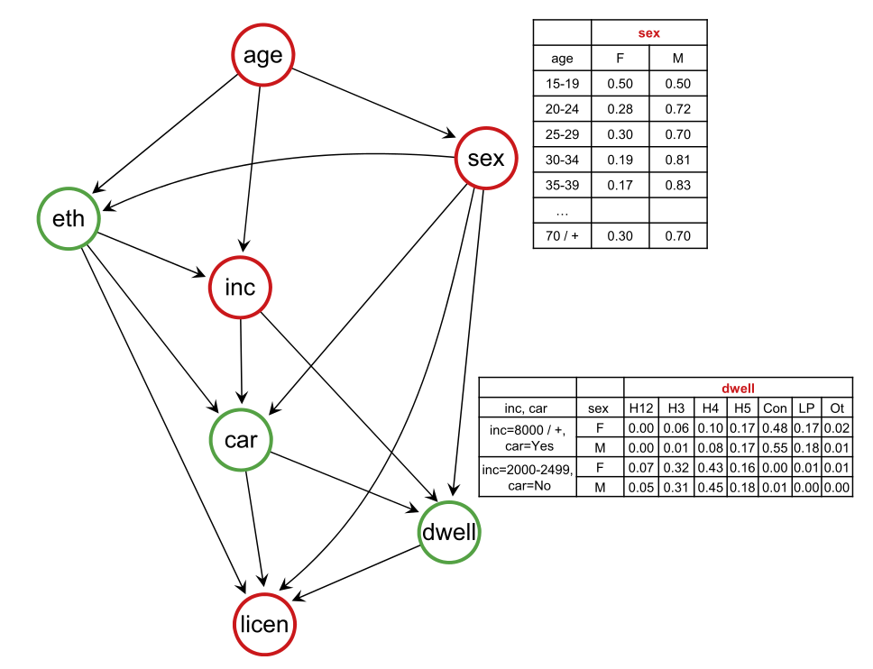
Sun, L., Erath, A., 2015. A Bayesian network approach for population synthesis. Transportation Research Part C: Emerging Technologies 61, 49–62. https://doi.org/10.1016/j.trc.2015.10.010
-
Population synthesis
The task is to create a synthetic representation of the population with socio-demographical households and person attributes
- Multitude of approaches
- Iterative Proportional Fitting (IPF)
- Iterative Proportional Updating (IPU)
- Gibbs Sampling
- Bayesian Networks
- Hidden Markov Models
Activity-based models
Saadi, I., Mustafa, A., Teller, J., Farooq, B., Cools, M., 2016. Hidden Markov Model-based population synthesis. Transportation Research Part B: Methodological 90, 1–21. https://doi.org/10.1016/j.trb.2016.04.007
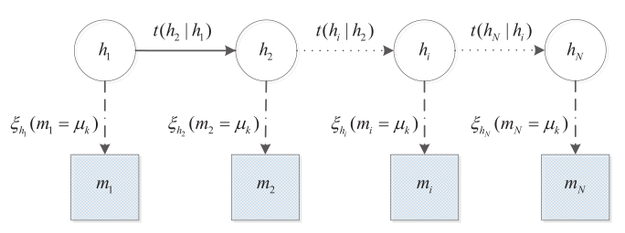
-
Population synthesis
The task is to create a synthetic representation of the population with socio-demographical households and person attributes
- Multitude of approaches
- Iterative Proportional Fitting (IPF)
- Iterative Proportional Updating (IPU)
- Gibbs Sampling
- Bayesian Networks
- Hidden Markov Models
- Deep Generative Modeling
Variational Auto Encoders
Activity-based models
Borysov, S.S., Rich, J., Pereira, F.C., 2019. How to generate micro-agents? A deep generative modeling approach to population synthesis. Transportation Research Part C: Emerging Technologies 106, 73–97. https://doi.org/10.1016/j.trc.2019.07.006
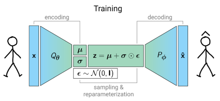
-
Synthesis of activity chains
Given sociodemographic attributes, generate daily activity chains for the agents.
- Today increasingly use of GPS / GSM trace data sets to train models
- Some examples
- Statistical Matching Approaches
- Skeleton-based approaches
- Sequential choice models (classic approach)
- Sequential Alignment Methods (SAM)
- Bayesian Networks
- ...
Activity-based models
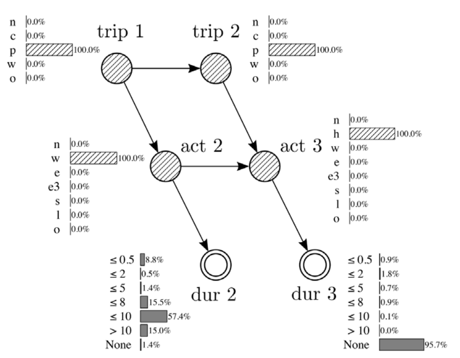
Joubert, J.W., de Waal, A., 2020. Activity-based travel demand generation using Bayesian networks. Transportation Research Part C: Emerging Technologies 120, 102804. https://doi.org/10.1016/j.trc.2020.102804
-
Further aspects:
- Departure times from activities
- Locations of activities
- Potential Path Areas (PPA)
- Space-time prisms
- ...
Activity-based models
Yoon, S.Y., Deutsch, K., Chen, Y., Goulias, K.G., 2012. Feasibility of using time–space prism to represent available opportunities and choice sets for destination choice models in the context of dynamic urban environments. Transportation 39, 807–823. https://doi.org/10.1007/s11116-012-9407-8
- As is demand generation, mobility simulation is often also more complex
- Usually agent-based
- Microscopic simulation
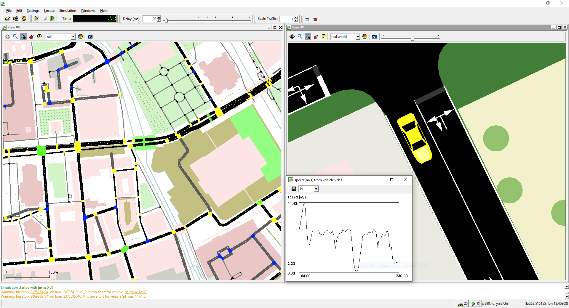
- VISSIM, SUMO, ...
- VISSIM, SUMO, ...
- Mesoscopic simulation
- MATSim, SimMobility,
POLARIS, ...
- MATSim, SimMobility,
Activity-based models
- Convergence
- Usually based on utility maximization principle
- Detection of Nash equilibria
- Output metric convergence
- Calibration
- Complex simulator (no closed form expression)
- Noisy output (needs stochastic optimization)
- Large run-times
Activity-based models: Challenges
Activity-based models: Examples
Timeline
- Lectures
- 10/01 8h30: Examples of large-scale models in transportation
- 10/01 10h45: Modeling methods I
- 13/01 14h00: Modeling methods II
-
13/01 16h45: Introduction to the student project
- Project work
- 27/01 14h00 + 16h45: Intermediate results
- 09/02 14h00 + 16h45: Exchange with other groups
- 23/02 14h00 + 16h45: Final presentation
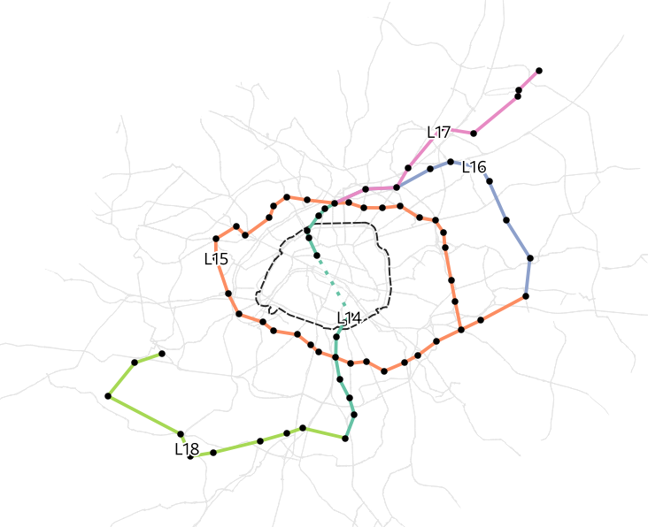
Grand Paris Express
- One of largest infrastructure projects in Europe
- Affecting mobility behaviour of large share of population in Île-de-France
Course project
- Learn more about Grand Paris Express
- Simple demand estimate for Grand Paris Express and its impact on existing public transport
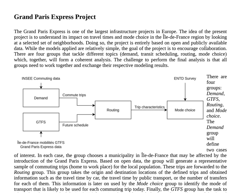
- Four groups:
- Demand
- Routing
- GTFS
- Mode choice
Please register for the groups:

Course project
Course: Grand Paris Express Project (2023)
By Sebastian Hörl
Course: Grand Paris Express Project (2023)
Université Gustave Eiffel


