Discrete choice modeling in transportation
HeadsUp Meeting
Sebastian Hörl
3 February 2023
Transport simulation
Transport simulation


Classic transport planning
- Zones
- Flows
- Peak hours
- User groups
Aggregated
Individual-based transport planning


0:00 - 8:00
08:30 - 17:00
17:30 - 0:00
0:00 - 9:00
10:00 - 17:30
17:45 - 21:00
22:00 - 0:00


- Discrete locations
- Individual travelers
- Individual behaviour
- Whole day analysis
Disaggregated
Icons on this and following slides: https://fontawesome.com
Demand generation

Population census (RP)
Income data (FiLoSoFi)
Commuting data (RP-MOB)
National HTS (ENTD)
Enterprise census (SIRENE)
OpenStreetMap
GTFS
Address database (BD-TOPO)

EDGT
Demand generation
Population census (RP)
Income data (FiLoSoFi)
Commuting data (RP-MOB)
National HTS (ENTD)
Enterprise census (SIRENE)
OpenStreetMap
GTFS
Address database (BD-TOPO)
EDGT
Open
Data

Open
Software
+
=
Reproducible research
Integrated testing
Demand generation
Population census (RP)
Income data (FiLoSoFi)
Commuting data (RP-MOB)
National HTS (ENTD)
Enterprise census (SIRENE)
OpenStreetMap
GTFS
Address database (BD-TOPO)
EDGT
Open
Data
Open
Software
+
=
Reproducible research
Integrated testing
Demand generation


Demand generation

Balac, M., Hörl, S. (2021) Synthetic population for the state of California based on open-data: examples of San Francisco Bay area and San Diego County, presented at 100th Annual Meeting of the Transportation Research Board, Washington, D.C.
Sallard, A., Balac, M., Hörl, S. (2021) Synthetic travel demand for the Greater São Paulo Metropolitan Region, based on open data, Under Review
Sao Paulo, San Francisco Bay area, Los Angeles five-county area, Switzerland, Montreal, Quebec City, Jakarta, Casablanca, ...
Transport simulation
Synthetic demand
Transport simulation
Mobility simulation
Synthetic demand
MATSim / SUMO / ...
See Seminar@SystemX by Ludovic Lerclecq
Transport simulation
Decision-making
10:00 - 17:30
17:45 - 21:00
22:00 - 0:00
Mobility simulation
Synthetic demand
Transport simulation
Decision-making
Mobility simulation
Synthetic demand
Transport simulation
Decision-making
Mobility simulation
Analysis
Synthetic demand
Transport simulation
Decision-making
Mobility simulation
Analysis
Synthetic demand
This seminar
Choice modeling


Images: Google Maps
General idea
General idea
Images: Google Maps
General idea


Images: Google Maps
General idea
Images: Google Maps
General idea
Images: Google Maps
General idea
Images: Google Maps
General idea


Images: Google Maps
General idea
Images: Google Maps
General idea
Images: Google Maps
General idea
- What should I choose? Or:
- What do people statistically choose?
Images: Google Maps
General idea
- Question: Given certain trip characteristics (travle times, costs, ...) for multiple mode, which mode would a person choose?
- A discrete choice between multiple alternatives.
- Here: Focus on mode choice, but other choices are relevant, for instance route choice or mobility tool ownership (cars, subscriptions, ...)
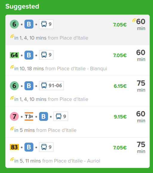
City Mapper
Survey data
Stated preference data
Felix Becker, Institute for Transport Planning and Systems, ETH Zurich.
Felix Becker, Institute for Transport Planning and Systems, ETH Zurich.
Stated preference data
Felix Becker, Institute for Transport Planning and Systems, ETH Zurich.
- Multiple choice situations
- Characteristics are varied multiple times
- Allows to estimate trade-offs between decisions
- Potential combinations of trip characteristics leads to an explosion of alternatives
- Need for efficient survey design methods
- Do certain preferences not show up in the behavioral models because they don't exist or the design doesn't catch them?
- Interesting literature on response burden
- How can the number of questions and their complexity be related to the number of persons actually doing the survey?
Stated preference data
Felix Becker, Institute for Transport Planning and Systems, ETH Zurich.
- Representativeness
- Need for oversampling when sending out the surveys (to catch traditionally less cooperative groups)
- Need for oversampling when sending out the surveys (to catch traditionally less cooperative groups)
- Robustness against misbehavior
- What if some people always choose the first option? (To win the incentive, for instance)
- What if some people always choose the first option? (To win the incentive, for instance)
- Main properties: All alternatives are fully known to the modeler and also to the decision-maker.
Revealed preference data
- Recorded trips (start time, end time, locations, ...)
- Many countries / territories perform Household Travel Surveys
- Recently more and more research on mobility traces (GPS, GSM)
- Stop detection, mode detection, ...
- Stop detection, mode detection, ...
- Main properties: Only one chosen alternative is reported and not all alternatives may have been known fully to the decision-maker.
- When estimating a behavioral model, we want to know WHY the decisions has been made. Hence, there is a need for choice set generation that reconstructs the characteristics of all alternatives that have been available in a specific situation.
Revealed preference data
- Various data sets are available in France
- Île-de-France
- Enquête Globale de Transport (EGT)
- (2010, on request); (2015 on yet published)
- Nantes, Lyon, Lille, ...
- Enquête Déplacements Grand Territoire (EDGT)
- Standardized (almost ;-) by CEREMA
- Available for various years depending on city
- Sometimes publicly accessible as open data (Nantes, Lille)
- France
-
Enquête Nationale Transports et Déplacements (ENTD)
- From 2008, available as open data
-
Enquête Mobilité des Personnes (EMP)
- From 2018, available as open data
-
Enquête Nationale Transports et Déplacements (ENTD)
- Île-de-France
Revealed preference data
-
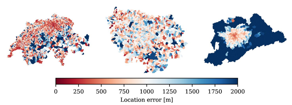
Challenge: Reconstruction of spatial anonymized surveys
- If Euclidean distances are available and spatial zones are not too large, respresentative (not the original) coordinates can be reconstructed
Summary on data
- Additional information in both SP and RP can be imputed per choice situation, for instance
- Population density at the origin / destination
- Distance to the closest transit stop at the origin / destination
- Income level of the decision-maker
- Age of the decision maker ...
- This information can be used in the modeling process.
-
SP usually gives models with a higher explanatory power, but requires a lot of expertise (survey design), funding (incentives, letters, platforms, ...), and time (between sending and response)
-
RP usually carries substantially more noise, but given data availability, can be applied in a relatively simple fashion, with large potentials for automatic data collection in the future.
- Finally, SP and RP data for the same context can be pooled, and some models even allow to obtain the relative explanatory power during the estimation process.
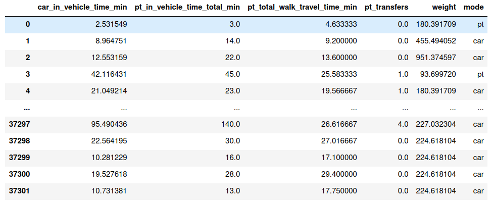
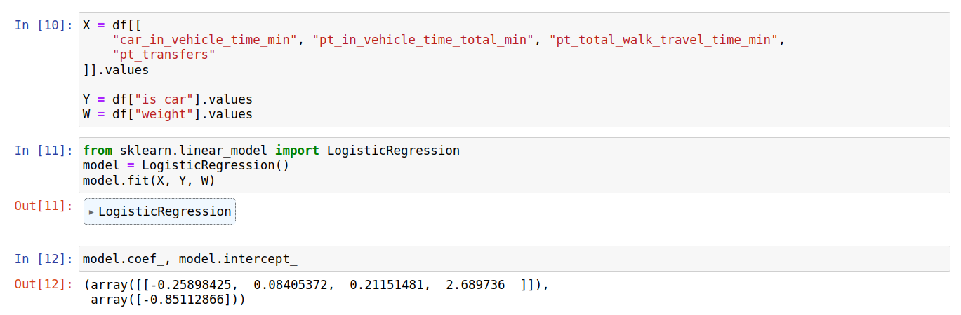
Parameter free models
General classification task
- The behavioral modeling task is relatively easy to accomplish with today's modeling libraries.
?
Attributes
Label
General classification task
- The behavioral modeling task is relatively easy to accomplish with today's modeling libraries.


General classification task
- The behavioral modeling task is relatively easy to accomplish with today's modeling libraries.
General classification task
- Limited ability to explain the choices
- Limited value for economic theory
- Elasticities
- How to generalize to new modes of transport (i.e. an additional label)?
Discrete choice models
Utility maximization
- Based on the homo oeconomicus concept: Decisions aim at maximizing a well-defined and quantified utility of the alternatives:
- v is the utility of alternative k (out of K existing ones)
- x are the characteristics of alternative k
-
β are the choice parameters
- The utility maximization models assumes that a rational decision-maker will choose alternative k with the highest utility:
v_k = \beta_{1} \cdot x_{1} + \beta_{2} \cdot x_{2} + ...
k^* = \text{arg max}_k \{ v_1, ..., v_k, ... v_K \}
Utility maximization: Example
-
Example: Choice between two public transport connections
v_k = \beta_\text{travelTime} \cdot x_{k, \text{travelTime}} + \beta_\text{interchanges} \cdot x_{k, \text{interchanges}}
Connection A
x_{A, \text{travelTime}} = 20\ \text{min}
Connection B
x_{B, \text{travelTime}} = 30\ \text{min}
x_{B, \text{interchanges}} = 0
x_{A, \text{interchanges}} = 1
-0.6
-1.0
-0.6 * 20 - 1.0 * 1 = -13
-0.6 * 30 - 1.0 * 0 = -19
Utility Maximization
- How can we estimate such a model?
- First we need decisions from N decision-makers indicated by i.
- We have registered choice characteristics
- We have the selected alternative
- We have the individual utilities (in vector form)
- Now the task is:
Find
\beta^*
such that
X_i
v_k(X_i) = \beta_k^T \cdot X_i
y_i
y_i = \text{arg max}_k \{ v_k(X_i\ |\ \beta^*) \} \ \
\forall i
Utility Maximization
- How can we estimate such a model?
- First we need decisions from N decision-makers indicated by i.
- We have registered choice characteristics
- We have the selected alternative
- We have the individual utilities (in vector form)
- Now the task is:
Find
\beta^*
such that
y_i = \text{arg max}_k \{ v_k(X_i\ |\ \beta^*) \} \ \
\forall i
X_i
v_k(X_i) = \beta_k^T \cdot X_i
y_i
Random Utility Model (RUM)
- Idea: We can model uncertainty (noise) explicitly in the decision-making process!
- Based on the systematic utility we define the random utility:
- Straightforward interpretation: Choices are sometimes perceived as better or worse, so on a large sample, we can assume fluctuations following a normal distribution
- The most attractive choice can be defined as
- Is this better?
u_{k,i} = v_{k,i} + \sigma \epsilon_{k,i}
\text{E}[\epsilon_{k,i}] = 0
\sigma \geq 0
with
k_i^* = \{ k \ | \ (u_{k,i} \geq u_{1,i}) \land \ (u_{k,i} \geq u_{2,i}) \land ... \}
Multinomial Logit Model (MNL)
- Is this better? Yes, but we need a special case!
- Choosing a normal distribution using an Extreme Value Distribution (e.g. Gumbel) ...
- ... leads to a closed-form expression of the choice probability:
\epsilon_{k,i} \sim \text{EV}
(Lots of math)
[Daniel McFadden in the 70s]
u_k = v_k + \sigma \epsilon_k
P[k] = \frac{\exp\left(\sigma^{-1}v_k\right)}{\sum_{k'}\exp\left(\sigma^{-1}v_{k'}\right)}
Multinomial Logit Model (MNL)
- Is this better? Yes, but we need a special case!
- Choosing a normal distribution using an Extreme Value Distribution (e.g. Gumbel) ...
- ... leads to a closed-form expression of the choice probability:
\epsilon_{k,i} \sim \text{EV}
(Lots of math)
[Daniel McFadden in the 70s]
P[k] = \frac{\exp\left(\sigma^{-1}(\beta_1 x_{k,1} + \beta_2 x_{k,2} + ...\right)}{\sum_{k'}\exp\left(\sigma^{-1}(
\beta_1 x_{k',1} + \beta_2 x_{k',2} + ...
)\right)}
u_k = v_k + \sigma \epsilon_k
Multinomial Logit Model (MNL)
- Is this better? Yes, but we need a special case!
- Choosing a normal distribution using an Extreme Value Distribution (e.g. Gumbel) ...
- ... leads to a closed-form expression of the choice probability:
\epsilon_{k,i} \sim \text{EV}
(Lots of math)
[Daniel McFadden in the 70s]
P[k] = \frac{\exp\left(\sigma^{-1}(\beta_1 x_{k,1} + \beta_2 x_{k,2} + ...\right)}{\sum_{k'}\exp\left(\sigma^{-1}(
\beta_1 x_{k',1} + \beta_2 x_{k',2} + ...
)\right)}
- Two alternatives:
Binomial logit model
- Multiple alternatives:
Multinomial logit model
u_k = v_k + \sigma \epsilon_k
Maximum likelihood estimation
- Coming back to estimation:
- How well does the model explain the taken choices? We can write a (log-)likelihood for this:
- Writing it out is quite simple, and you will see that it is at least twice differentiable. Additionally, McFadden (again!) has proven that the log-likelihood is concave. This means maximizing the log-likelihood is easy. It gives us the Maximum Likelihood Estimate (MLE) for β!
- It can be found using standard methods such as gradient descent or Newton-Raphson.
\pi(k|\beta) = \frac{\exp(\sigma^{-1} v_k)}{\sum_{k'}\exp(\sigma^{-1} v_{k'})}
v_k(X_i) = \beta^T \cdot X_k
y_i \in \{ 1, ..., K \}
\mathcal{L}(\beta|y_{1:N}) = \prod_i \pi(y_i | \beta)
\mathcal{l}(\beta|y_{1:N}) = \sum_i \log( \pi(y_i | \beta) )
\hat \beta_{MLE} = \argmax_{\beta} \mathcal{l}(\beta|y_{1:N})
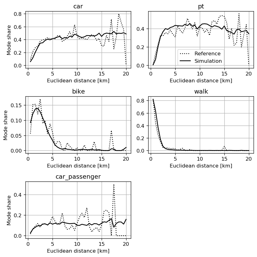
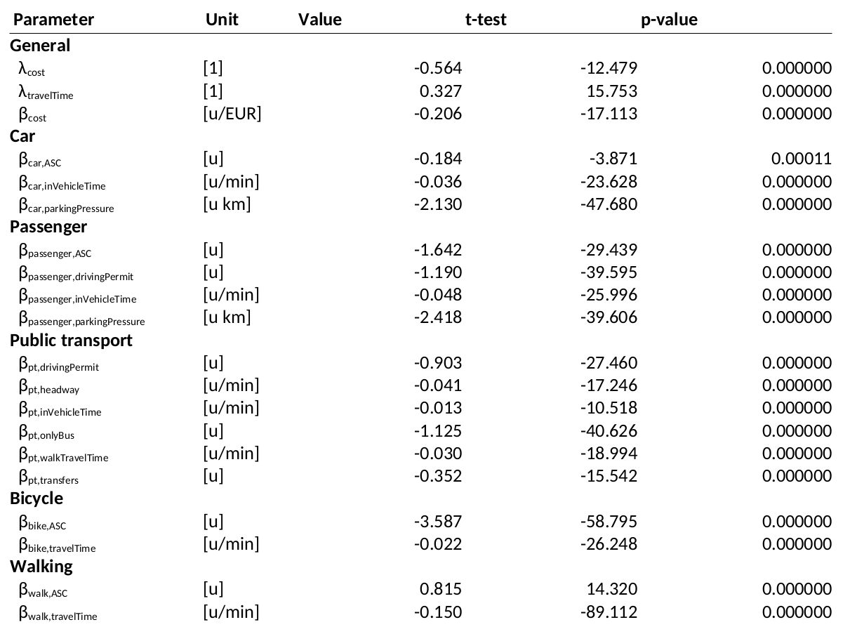
Example results
R2 = 0.52
Example results
R2 = 0.52
Example results
R2 = 0.52
Example results
R2 = 0.52
Example results
R2 = 0.52
Example results
R2 = 0.52
Details on statistical tests (for those interested)
- Two-sided Student's t-test is used to test whether a parameter β is significantly different from zero on confidence level α:
- How do we obtain the estimated standard deviation? This is unfortunately usually not explained when introducing the MNL.
- The Observed Fisher Information Matrix in MLE is the Hessian of the log-likelihood (or score function) evaluated at the ML estimate. The diagonals represent the uncertainty on the parameters:
\frac{\alpha}{2} \leq t\left(
\frac{\hat \beta_{u,MLE}}{\hat \sigma_u}
\right) \leq 1 - \frac{\alpha}{2}
\hat F = \sqrt{
\frac{\partial^2 l(\beta)}{\partial \beta^2} \left( \hat \beta_{MLE} \right)
}
\hat \sigma_u = \hat F_{uu}
Interpretation
Model selection
- What is the R2 of the model? Does it increase / decrease if variables are added / removed?
- Are the signs of the parameters coherent? Do they point in the right direction (for instance, increasing travel time should decrease utility).
- Are the magnitudes of the parameters coherent? Does one variable have unrealistically more influence than another one?
Elasticities
- The estimated model defines the probability of choosing mode k given certain choice characteristics (X) and the estimated model parameters:
- An elasticity in economics describes how an output quantity changes when an input quantity is altered. Here: How does the probability change if a certain choice characteristics change?
- In economics, more often defined in terms of percentage.
- Used to compare between models in different contexts. Often relatively stable!
\pi(k) = \frac{\exp\left(\hat \beta^T \cdot X\right)}{\sum_{k'}\exp\left(\hat \beta^T \cdot X\right)}
\frac{\partial \pi_A(u_k)}{\partial x_A} = \ ?
Direct elasticity
Cross elasticity
\frac{\partial \pi_A(u_k)}{\partial x_B} = \ ?
Black box
- Difficult to estimate, only a posteriori
- DebiAI?
Value of Travel Time Savings
-
Utility is an abstract mathematical concept. On the contrary, most choice characteristics have a unit, for instance distance, travel time, money.
- Let's redefine , i.e. we transform all parameters into a new space
- With we get the Value of Travel Time Savings
v = \beta_\text{travelTime} \cdot x_\text{travelTime} \\
+ \beta_\text{cost} \cdot x_\text{cost}
[1/min] * [min]
[1/EUR] * [EUR]
\beta_u = \tilde \beta_u \cdot A
A = \beta_{cost}
\tilde \beta_\text{travelTime} = \beta_\text{travelTime} / \beta_{cost}
\tilde \beta_\text{cost} = 1
[EUR/min]
[1]
Value of Travel Time Savings
- The Value of Travel Time Savings (VTTS) explains how much money persons (on average) would be willing to pay extra if the travel time on a specific connection is reduced by a certain amount of time.
- Other interpretation: How uncomfortable is it to spend a certain duration in one mode of transport vs. another one? The VTTS is the higher, the more "costly" or uncomfortable it is to take a trip using this transport mode.
- VTTS are relatively stable over different surveys and countries after accounting for the respective currencies.
VTTS = \tilde \beta_\text{travelTime} = \beta_\text{travelTime} / \beta_{cost}
Value of Travel Time Savings


13 CHF/h
AMoD
Taxi
19 CHF/h
Conventional
Car
12 CHF/h
Public
Transport
AMoD
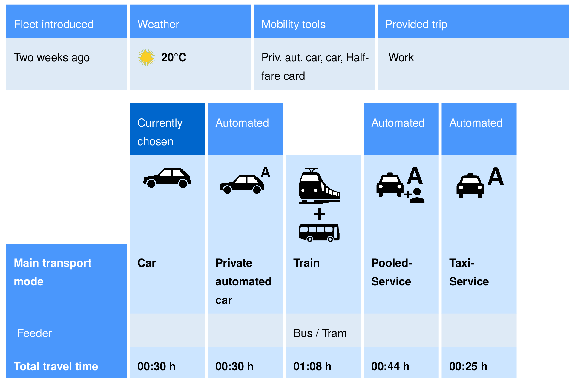
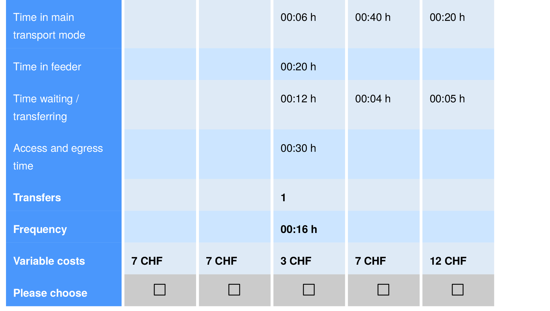
- Remember the survey from before on the introduction of automated taxis in the transport system of Zurich?
Value of Travel Waiting Time Savings
13 CHF/h
AMoD
Taxi
19 CHF/h
Conventional
Car
12 CHF/h
Public
Transport
AMoD
- Remember the survey from before on the introduction of automated taxis in the transport system of Zurich?

21 CHF/h
32 CHF/h
Value of Travel Waiting Time Savings
13 CHF/h
AMoD
Taxi
19 CHF/h
Conventional
Car
12 CHF/h
Public
Transport
AMoD
- Remember the survey from before on the introduction of automated taxis in the transport system of Zurich?
Black box
- VTTS only measurable because of linear structure of the utilities
21 CHF/h
32 CHF/h
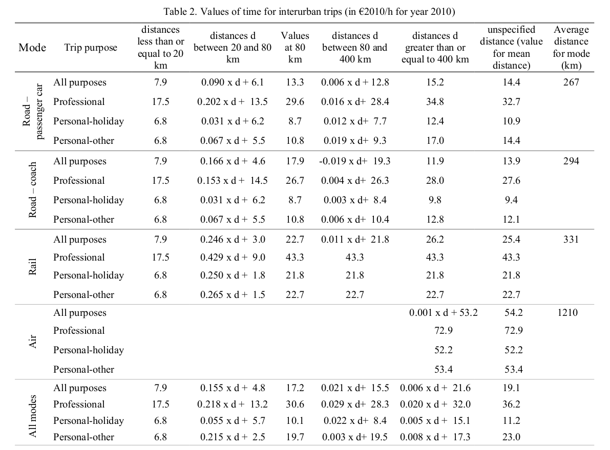
Cost benefit analysis
- What is the value of decreasing the travel time Paris <> Clermont by 30 minutes?
- Standardized VTTS, for instance (Meunier & Quinet, 2015)
- VTTS = 21.8 EUR/h
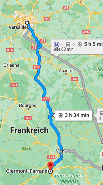
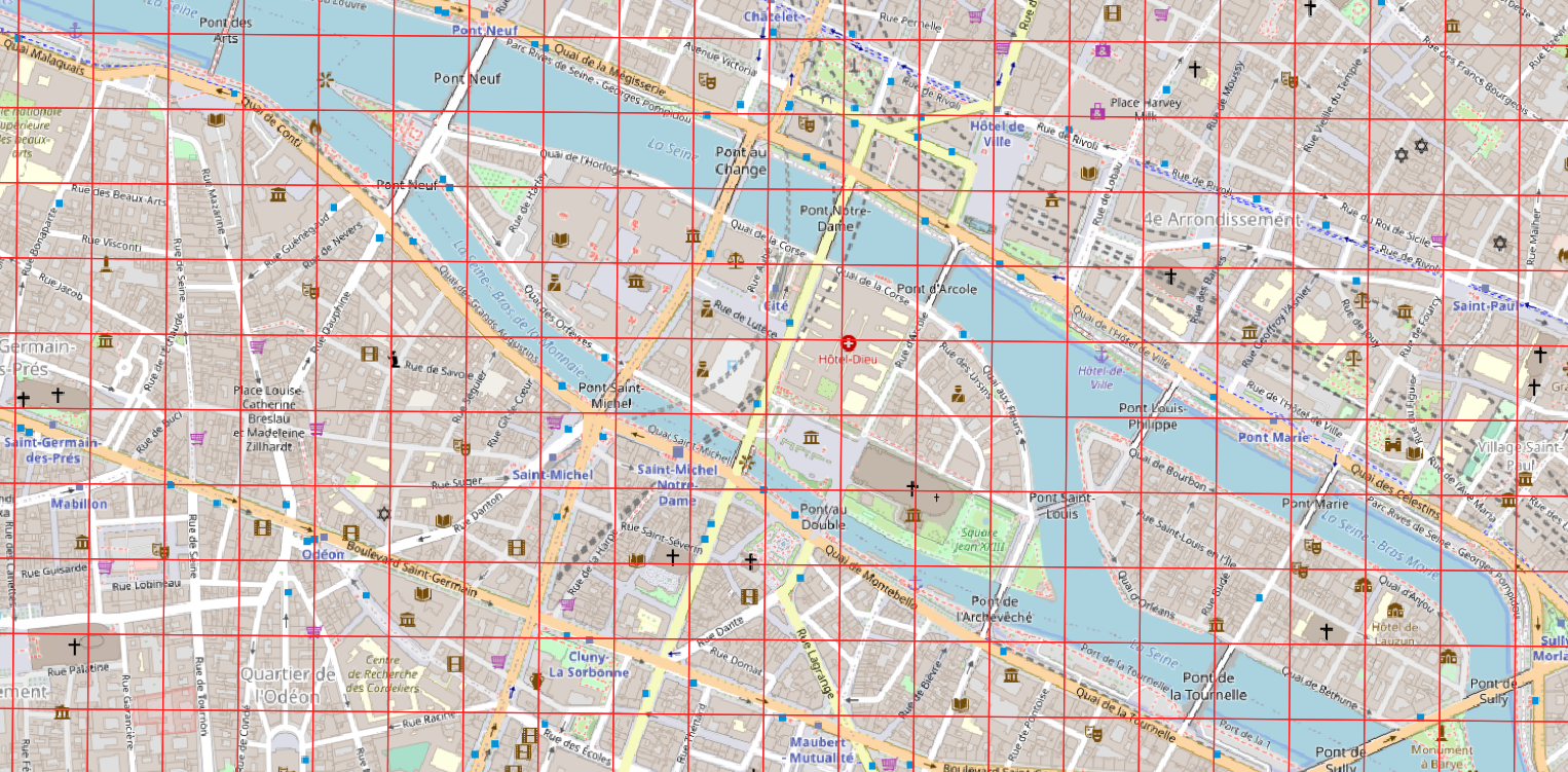
Google Maps
Simulation
- Given a new choice situation X we can now simulate the choice outcome.
-
Option 1: Sampling
- Calculate systematic utilities
- Calculate probabilities
- Sample one alternative
- Calculate systematic utilities
v_k(X)
\pi_k(v_k)
y \sim \pi_k(v_k)
Simulation
- Given a new choice situation X we can now simulate the choice outcome.
-
Option 2: Maximum selection
- Calculate systematic utilities
- Sample an errors terms
- Select the maximum
- Calculate systematic utilities
v_k(X)
\epsilon_k \sim \text{Gumbel}
y = \text{arg max}_k \left\{
v_1 + \epsilon_1, ..., v_K + \epsilon_K
\right\}
Simulation
- Side note: These approaches may generate a different outcome every time the choice is taken. In our agent-based simulations, we often simulate multiple days of the same persons. To increase stability, we would like to get the same outcome if the choice characteristics stay constant.
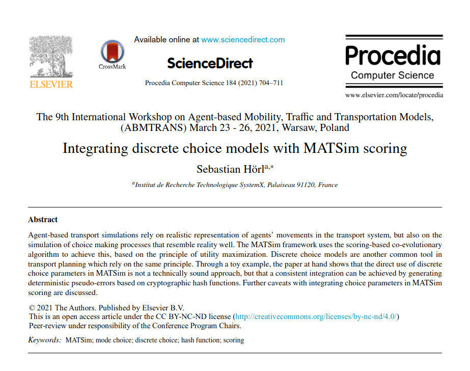
- Idea: Assign deterministic error terms to every trip + mode combination that, as an ensemble follow the respective EV distribution.
- Makes use of the avalanche effect in hash functions to generate errors that are a deterministic function of the input (trip and mode)
New choices
- How can we add new modes of transport (for which we do not have survey data)?
- Hypothesize the systematic utility of the mode.
- Can we transfer values (as they have a specific meaning) from one mode to another?
- For instance, autonomous taxis are similar to public transport. As a first guess, we can assume that waiting time is valued similarly to public transport. The same goes for the travel time.
- Hypothesize the systematic utility of the mode.
- Standard approach when no survey data is available!
Black box
- Not clear how to easily generalize to new modes of transport
Variations / Additions
Availability of alternatives
- Sometimes, an alternative is not available at all for a specific choice situation. Including availabilities is straight-forward in an MNL and the respective log-likelihood.
- Examples:
- Car is not available for trips with persons under 18 years (person attribute)
- Car is not available for trips with persons without a license (person attribute)
- Car is not available for trips without cars in the household (household attribute)
- Public transport is not available if the next stop is further than 5km
- ...
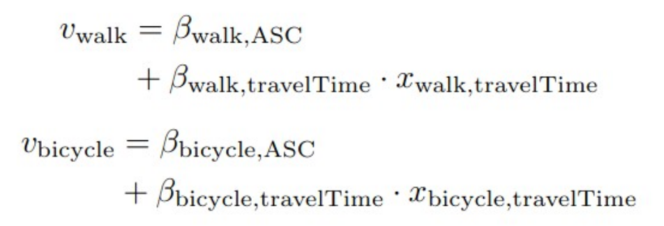
- Ideally (for most modeling software) one alternative must always be available, usually walking
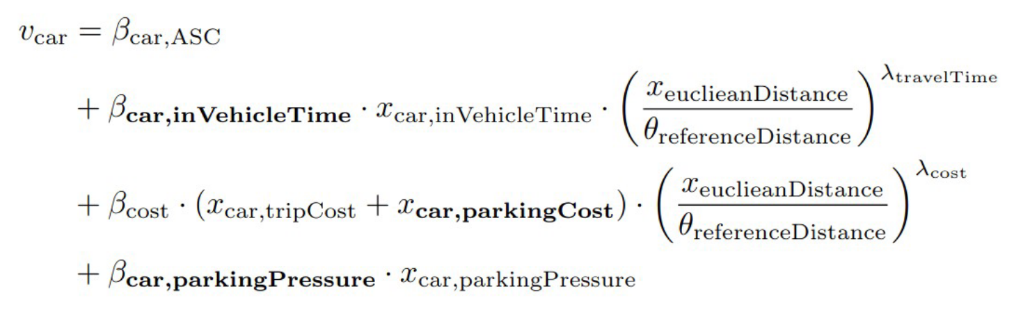
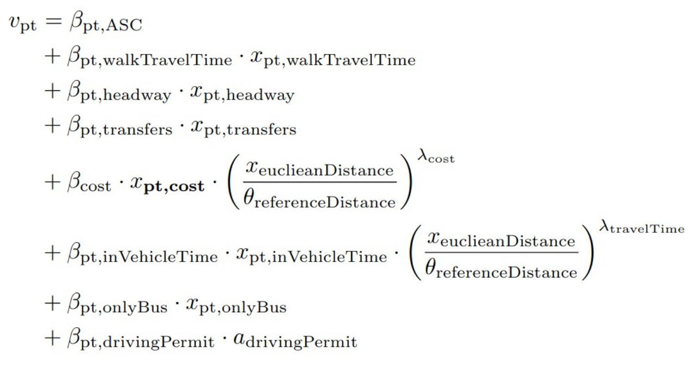
Interaction terms
- Surveys have shown that the perception of costs varies based on distance. The standard MNL formulation allows to easily integrate interaction terms:
- θ is an arbitrary constant (usually the average, e.g. the average Euclidean distance) that acts as a reference for the interaction term
- λ is estimated along with the β as a model parameter and usually negative
- Meaning that the travel time has lower influence on the choice for longer distances than for shorter ones
v_{car} = \beta_\text{travelTime} \cdot \left(
\frac{x_\text{euclideanDistance}}{\theta_\text{euclideanDistance}}
\right)^\lambda \cdot x_\text{travelTime} + ...
Interaction terms
- Second example: With increasing income level of the person, the impact of cost on the choice diminishes:
- θ is the average income of the population
- Interactions can be arbitrarily combined (multiplied)
v_{car} = \beta_\text{cost} \cdot \left(
\frac{x_\text{income}}{\theta_\text{income}}
\right)^\lambda \cdot x_\text{cost} + ...
Many other aspects
- There is a large field of discrete choice modeling with specific journals (Journal of Choice Modeling)
- What happens if we replace the EV distribution by a Normal?
- I get a Multinomial Probit model
- No analytical likelihood function anymore; simulation stays straight-forward
- Possibility to flexibly model the error term
- Correlations between choice alternatives
(if I like the red bus, I also like the blue bus)
- More complex formulations of the MNL exist
- Mainly to disentangle the above-mentioned correlation structure of errors
- Nested logit model (first I choose that I use the bus, then if I prefer red or blue)
-
Cross-nested logit model (an automated taxi is like a bus, but also a bit like a car)
- Multiplicative error terms ...
- Parameters (β) are not static but follow a distribution themselves ...
Finally, making use of deep learning :)
- Usually, the models contain Alternative Specific Constants (ASC) which capture the unexplained systematic variation. These are things that are not modeled in the systematic utility.
- What if we make these ASCs dependent on external inputs (person's age, income, ...) and model them using a DNN?
- Current research, e.g. Bierlaire et al.
v_{car} = \beta_\text{ASC,car} + \beta_\text{travelTime,car}\cdot x_\text{travelTime} + ... \\
v_{pt} = \beta_\text{ASC,pt} + \beta_\text{travelTime,pt}\cdot x_\text{travelTime} + ...
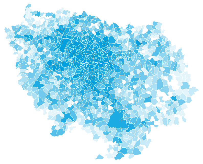
Île-de-France
Modeling process
Data cleaning
Car alternatives
Transit alternatives
Modeling
-
Enquête Globale de Transport 2010 for Île-de-France
- Four level HTS (Households, Persons, Trips, Stages)
- All households members have been interviewed (rare, with lots of potential!)
- For week days, 35k persons with 100k+ trips
- Data has already been weighted
- For each person, a whole day is described
- Activities (Location, types, durations, ...)
- Trips (Origin, destination, departure time, arrival time, mode of transport, ...)
- Locations are known on a grid of 100x100 meters (i.e. almost perfectly)
Modeling process
Data cleaning
Car alternatives
Transit alternatives
Modeling
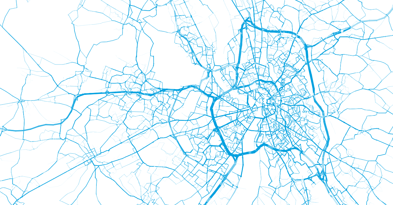
- Common approach: Use APIs such as HERE, Google, Bing to obtain travel times, but this is not easily replicable and reproducible
- We use OpenSteetMap data and perform a Dijkstra shortest path based on existing and imputed speed limits
- Added multiple factors
- From speed limits to freeflow travel time (x1.3)
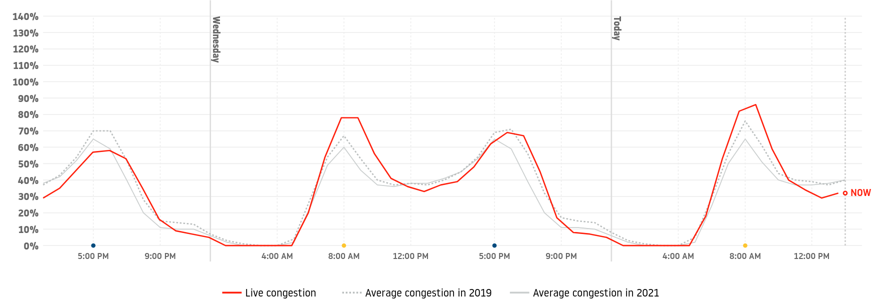
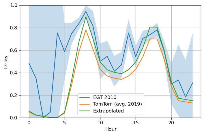
- From freeflow to congested travel time using TomTom Congestion Index
Modeling process
Data cleaning
Car alternatives
Transit alternatives
Modeling
- Common approach: Use APIs such as HERE, Google, Bing to obtain travel times, but this is not easily replicable and reproducible
- We use OpenSteetMap data and perform a Dijkstra shortest path based on existing and imputed speed limits
- Added multiple factors
- From speed limits to freeflow travel time (x1.3)
- From freeflow to congested travel time using TomTom Congestion Index
- From 2019 to 2010 using a scaling factor
- Good match with actual car trips in EGT
-
Cost model:
- 0.2 EUR/km
- Parking 3 EUR/h (Paris 2010)
Modeling process
Data cleaning
Car alternatives
Transit alternatives
Modeling
- Again, we could use an API for transit routing, but we want to be replicable
- Île-de-France Mobilités published regularly the full digital transit schedule in GTFS format for the whole region
- Used to perform transit routing using the RAPTOR algorithm
Origin
Destination
Round 1
Modeling process
Data cleaning
Car alternatives
Transit alternatives
Modeling
- Again, we could use an API for transit routing, but we want to be replicable
- Île-de-France Mobilités published regularly the full digital transit schedule in GTFS format for the whole region
- Used to perform transit routing using the RAPTOR algorithm
Origin
Destination
Round 2
-4
-1
-1
-0.2
Modeling process
Data cleaning
Car alternatives
Transit alternatives
Modeling
- Again, we could use an API for transit routing, but we want to be replicable
- Île-de-France Mobilités published regularly the full digital transit schedule in GTFS format for the whole region
- Used to perform transit routing using the RAPTOR algorithm
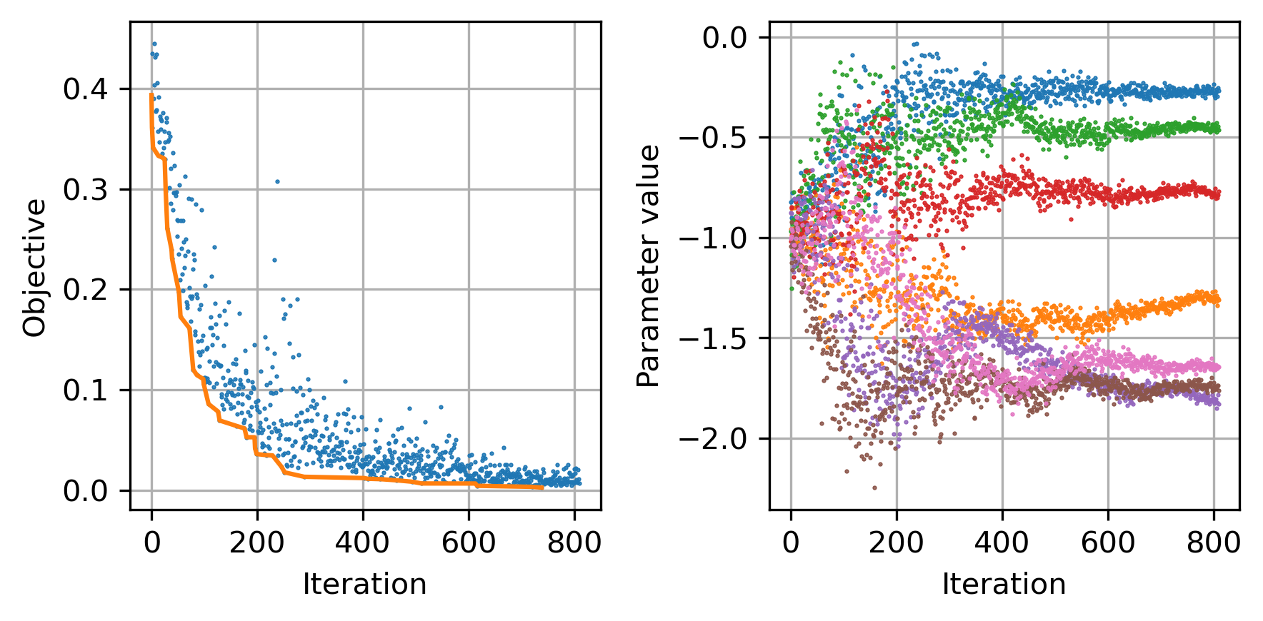
- Black box optimization (CMA-ES) of routing parameters to match overall transport mode share among all transit trips in the EGT
Modeling process
Data cleaning
Car alternatives
Transit alternatives
Modeling
- Again, we could use an API for transit routing, but we want to be replicable
- Île-de-France Mobilités published regularly the full digital transit schedule in GTFS format for the whole region
- Used to perform transit routing using the RAPTOR algorithm
- Black box optimization (CMA-ES) of routing parameters to match overall transport mode share among all transit trips in the EGT
-
Cost model (more complex)
- 0 EUR if the person has a public transport subscription
- 1.80 if origin and destination are within Paris OR if only Metro and Bus are used
- Otherwise, regression model from Abdelkader DIB (IFPen)

Distances: OP = Origin > Paris; DP = Destination > Paris; D = Direct
Modeling process
Data cleaning
Car alternatives
Transit alternatives
Modeling

Final model
Data cleaning
Car alternatives
Transit alternatives
Modeling
Parking
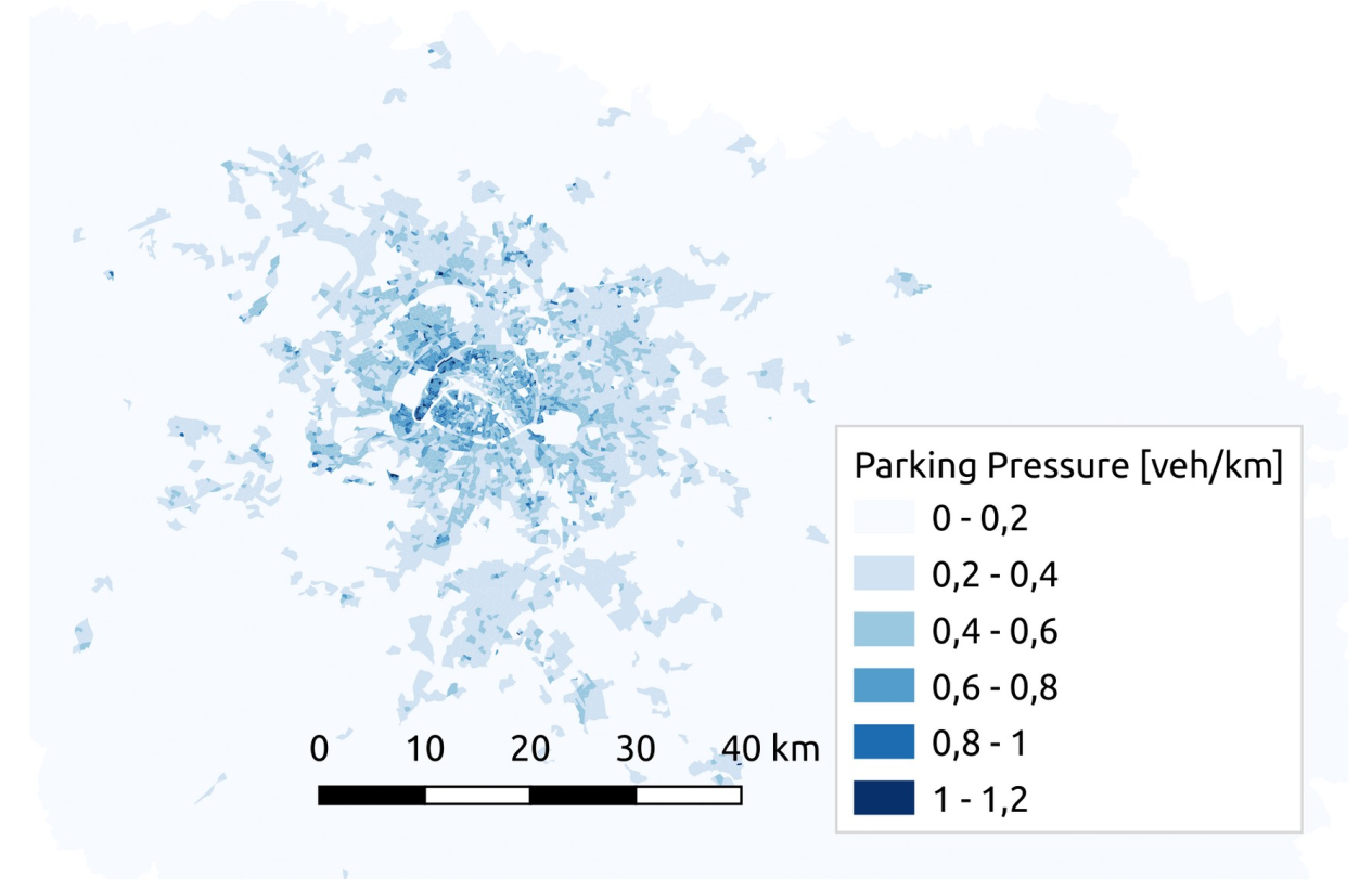
Parking pressure =
Total road length
Number of cars
Passengers
Next steps
Agent-based simulation
- Choice model has been implemented in our reference model for Île-de-France
- Currently, it is reusing a recalibrated choice model for Zurich
- First results look very promising
- Remaining work to calibrated speeds and capacities in the road network
-
Goal: Present a fully calibrated agent-based simulation of a large territory like Île-de-France that is fully replicable (synthetic population and simulation outcomes)
- Use case: Estimating the effect of the Grand Paris Express and optimal design of feeder services (project exploratoire 2023)
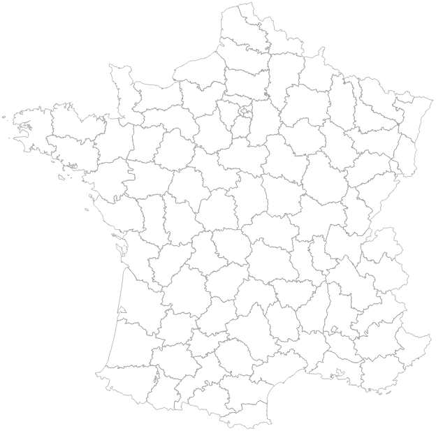
Transfer to other use cases
- Theoretically, the model can be transferred to other use cases in France (no IDF-specific variables are used)
- Practically, we have already cleaned HTS for Lyon, Nantes (and Lille) for our synthetic populations
- We have (partly) solved the spatial anonymization challenge
- Still some work to do to collect information (public transport costs, ...)
- Two options:
- Estimation of the same model case by case and then comparison of the outcomes (hopefully similar)
- Estimation of a joint model for French cities in general (large potential for generalization in our projects!)
- Estimation of the same model case by case and then comparison of the outcomes (hopefully similar)
Questions?
Discrete choice modeling in transport planning
By Sebastian Hörl
Discrete choice modeling in transport planning
IRT SystemX, HeadsUp, 3 February 2023


