Topics of Discussion

• Input Normalisation
• Weight Initialization Strategies
• Loss Functions
• Activation Functions
• Choice of Optimizers
• Dropout
• Optimizer Hyperparamters (learning rate, epochs, etc.)
• Model Hyperparameters (no. of hidden layers, hidden layer size, etc.)
• Batch Normalization

Structure of the Workshop

• Highlighting the problem
  
  
   
• A discussion of the technique that can address the problem
  
  
   
• Implementation in Code

Starting model

A benchmark network in keras.

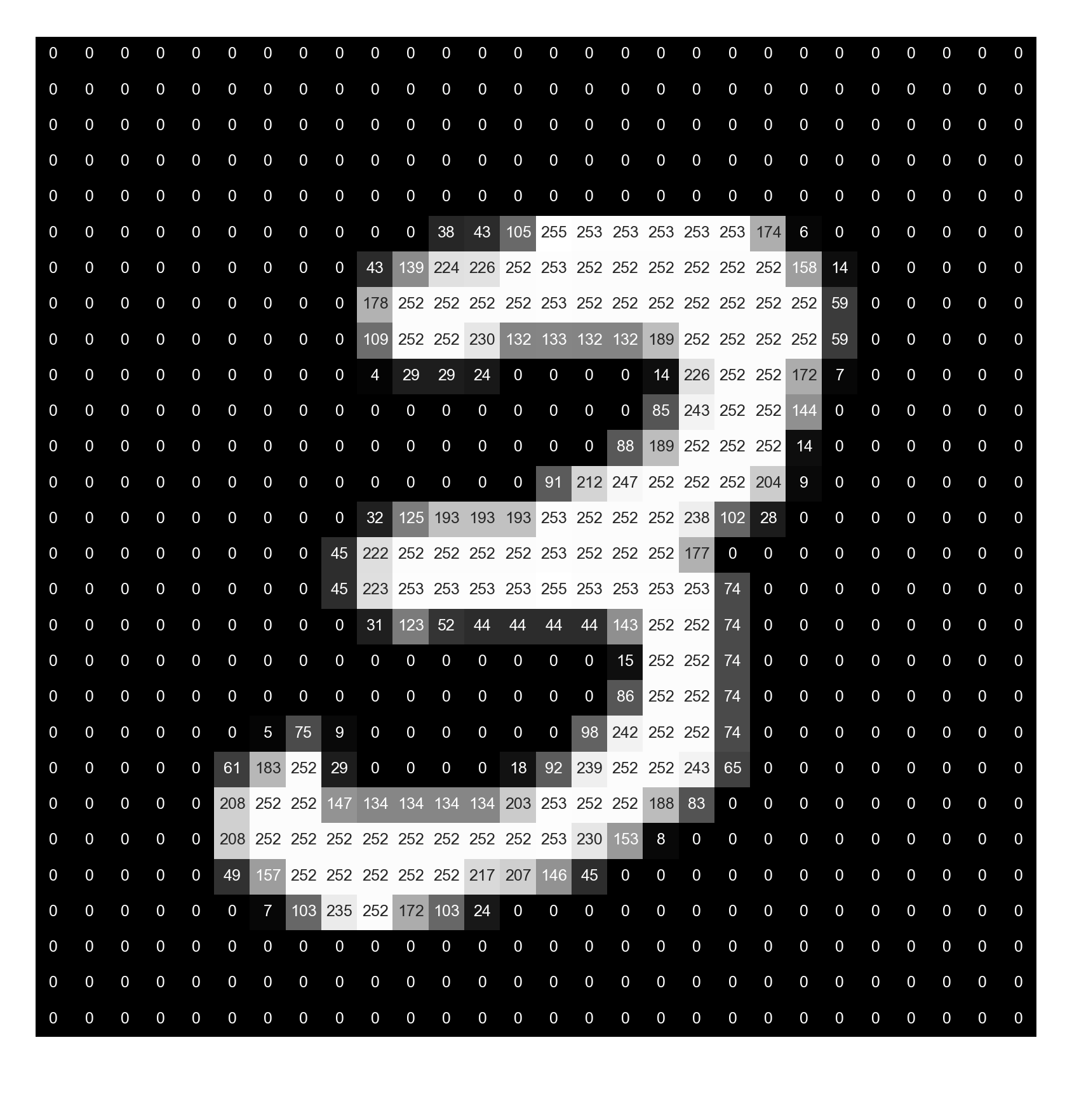
Dataset: MNIST

No. of hidden layers: 2

No. of hidden units: 10

from keras.datasets import mnist
from keras.models import Sequential
from keras.layers import Dense, Flatten, Activation
from keras.optimizers import SGD
from keras.utils import to_categorical
from matplotlib import pyplot as plt
import seaborn as sns

(x_train, y_train), (x_test, y_test) = mnist.load_data()

num_classes = 10

# Apply one-hot encoding to the labels
y_train = to_categorical(y_train, num_classes)
y_test = to_categorical(y_test, num_classes)

# Break training data into training and validation sets
(x_train, x_valid) = x_train[:50000], x_train[50000:]
(y_train, y_valid) = y_train[:50000], y_train[50000:]

# Model definition
model = Sequential()
model.add(Flatten(input_shape=(28,28)))

# Model hyperparameter
num_hidden_layers = 2
num_hidden_units = 10

for _ in range(num_hidden_layers):
    model.add(Dense(num_hidden_units))
    model.add(Activation('relu'))

# Output Layer
model.add(Dense(num_classes))
model.add(Activation('softmax'))

# Set optimization hyperparameters
batch_size = 256
epochs = 10

model.compile(
    optimizer='adam', 
    loss='categorical_crossentropy',
    metrics=['accuracy'])

history = model.fit(
    x_train, y_train, 
    epochs=epochs, 
    batch_size=batch_size,
    validation_data=(x_valid, y_valid), 
    verbose=2)

accuracy_score = model.evaluate(
    x_test, y_test, batch_size=128)

print(f'\nTest accuracy: {accuracy_score[1]:>5.3f}')

Epoch 1/10
1s - loss: 2.8814 - acc: 0.2122 - val_loss: 1.9508 - val_acc: 0.2677
Epoch 2/10
0s - loss: 1.9028 - acc: 0.2714 - val_loss: 1.8804 - val_acc: 0.2859
...
...
...
Epoch 10/10
0s - loss: 0.9046 - acc: 0.6434 - val_loss: 0.8798 - val_acc: 0.6495
 5632/10000 [===============>..............] - ETA: 0s
Test accuracy: 0.648

Model Evaluation

Input Normalisation

Rule of Thumb

Input values and activations should be small and not come from highly variable distributions.

Different units for features

• Features could be measured in different units - Kms and Kgs
• Normalization makes inputs uniform for all feature representations
• Large values lead to saturating gradients.
• Results in efficient training
• Min-Max Normalization and Z-Score Normalization

Min-Max Normalization

A is the overall range of values. [C, D] is the interval that we want to map to.

For the range [0, 1], The formula becomes:

Weight Initialization Strategies

The problem with improper weights

Strategies for initialization

• All zeros
• Sampling Normal Distribution ~ (0, 1)
• Sampling Normal Distribution ~ (0, 0.1)
• Xavier Initialization
• He Initialization

All Zeros

• Never  do this!
• All neurons output similar activations
• Similar gradients during backpropagation
• We need to break asymmetry between inputs

Sampling Normal Distribution ~ (0,1)

• Can result in the weighted inputs being large
• Saturating Neurons

tf.truncated_normal(shape=(INPUT, OUTPUT), mean=0, stddev=1)

Sampling Normal Distribution ~ (0,0.1)

• Weights concentrated near 0
• Efficient learning
• Can be used as the go-to strategy

tf.truncated_normal(shape=(INPUT, OUTPUT), mean=0, stddev=0.1)

Xavier Initialization

• Glorot & Bengio (2010)
• Sample Normal Distribution ~ (0, 1/N)
• Works well in many cases
• Not ideal for ReLu activations

W = tf.get_variable("W", shape=[INPUT, OUTPUT], initializer=tf.contrib.layers.xavier_initializer())

He Initialization

• Sample Normal Distribution ~ (0, 2/N)

W = tf.get_variable("W", shape=[INPUT, OUTPUT], initializer=tf.contrib.layers.variance_scaling_initializer())

Activation Functions

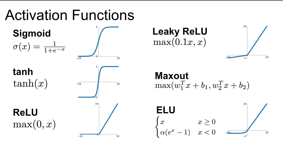
Activation Functions

Sigmoid

• The problem of vanishing gradient
• Output is not zero-centered
• Not a good choice for hidden layers
• Almost always applied at the final output layer (Binary Classification)

Activation Functions

Tanh

• The problem of vanishing gradient remains
• Output is zero-centered
• Not the ideal choice for hidden layers
• In practice, performs better than Sigmoid

Activation Functions

Rectified Linear Units (ReLu)

• Solves the problem of vanishing gradient
• Standard non-linearity for hidden layers
• Can suffer from 'dead' hidden units. 

Batch Normalization

Batch Normalization

• Normalizing inputs to all the layers of a network
• Normalization using mean and variance of the current mini-batch
• Inference happens using population mean and variance

Batch Normalization

• Network trains slower

• Helps with the problem of vanishing gradients

• Added job of regularizing the model

• Leads to faster convergence to optimal accuracy.

• Allows higher learning rates, faster training.

• Allows building much deeper networks.

Before Batch Normalization

After Batch Normalization

Dropout

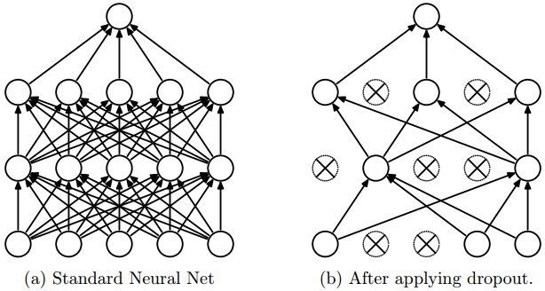
Image Source: http://http://cs231n.github.io

Dropout

• Main job is to prevent overfitting
• Works extremely well.
• Increases training time.
• Requires hyperparameter tuning (keep probability)

Choice of optimizers

• Optimal Learning rate
• Why use the same learning rate for every parameter?
• Escape sub-optimal local minima
• Deal with Saddle points

Choice of optimizers

• GradientDescentOptimizer
   
• Momentum Optimizer
   
• AdagradOptimizer
   
• AdamOptimizer

Gradient Descent Optimizer

• The baseline optimizer
• Essentially used as the Stochastic Gradient Descent optimizer
• Only parameter to tune is learning rate

Momentum Optimizer

• Softens the update oscillations in irrelevant directions
• Adds a fraction of the past step update to the current one
• Parameter vector builds up velocity in the direction of consistent gradients
• Can overshoot minima - Use Nesterov Momentum

AdaGrad Optimizer

• Uses different learning rate for every parameter based on past gradients
• Parameters with high gradients will have learning rate reduced
• Weights with small/infrequent updates have their learning rates increased
• Disadvantage - Learning rates always decreasing
• Can lead to situation where no learning happens
• Rectified by AdaDelta Optimizer

Adam Optimizer

• Combines the best of AdaGrad and RMSProp
• AdaGrad works well for Sparse features and gradients
• Best performing optimizer

Optimizer Hyperparameters

• Learning Rate
   
• Momentum
   
• Mini-batch size
   
• Number of Epochs

Learning Rate

• The most important hyperparameter to tune.
• Larger values can make the model very unstable.
• Lower values take too long to converge.

Batch Size

Small

• Good for training.

• Smaller updates and longer training leads to lower overall error.

• Lower learning rates and more epochs means longer training times.

• Need to compensate with lower learning rates and more epochs

• Low memory usage.

Batch Size

Large

• High memory consumption.

• Lower number of weight updates will not let the network train effectively

• Faster training.

Epochs

• Need to stop training before network starts overfitting
• Use large values and checkpoint model training

Model Hyperparameters

• Number of Hidden Layers
  
   
• Number of Hidden Units

Number of Hidden Layers

• Helps increase the representative power of the model
   
• Increasing helps capture hierarchical structures better - e.g. CNNs

Number of Hidden Units

• Should be as large as possible - more parameters to tune
• Same size for all layers works better in practice
• Overcomplete layers better than undercomplete layers.

Batch Normalization