Kalman filter

History

Named by Rudolf E. Kálmán (*1930 Hungary)
First described in 1958-1961

Trajectory estimation for Apollo (NASA)
Navigation of nuclear ballistic missile submarines (US Navy)
Navigation systems of cruise missiles
Navigation systems of modern spacecrafts (Space Shuttle 2011)
Attitude control and navigation systems of the International Space Station (ISS)

G-H Filter

estimate = prediction + G(residual)

e s t i m a t e = p r e d i c t i o n + G (r e s i d u a l)

newG = oldG + H (\frac{residual}{timestep})

n e w G = o l d G + H (\frac{​ r e s i d u a l ​ ​}{​ t i m e s t e p ​})

residual = measurement - prediction

r e s i d u a l = m e a s u r e m e n t - p r e d i c t i o n

G-H Filter

estimates = [measurement]
predictions = []

for m in measurements:
    # prediction step
    prediction = prediction + behavior_model*time_step
    behavior_model=behavior_model

    predictions.append(prediction)
    
    # update step    
    residual = m - prediction    
    behavior_model = behavior_model + H * (residual/time_step)
    prediction    = prediction    + G * residual
  
    estimates.append(prediction)

Bad initial condition

Acceleration

Choosing of G

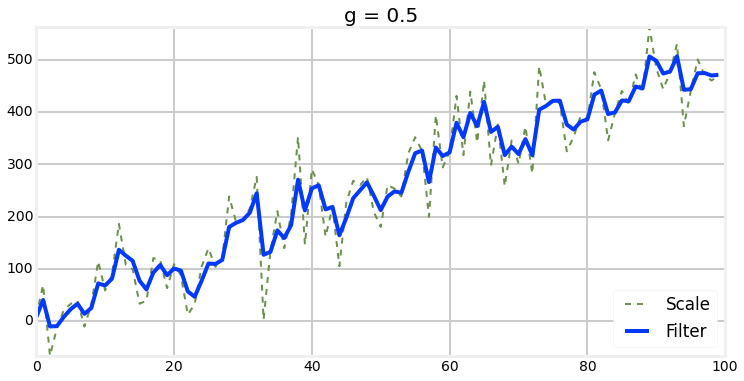
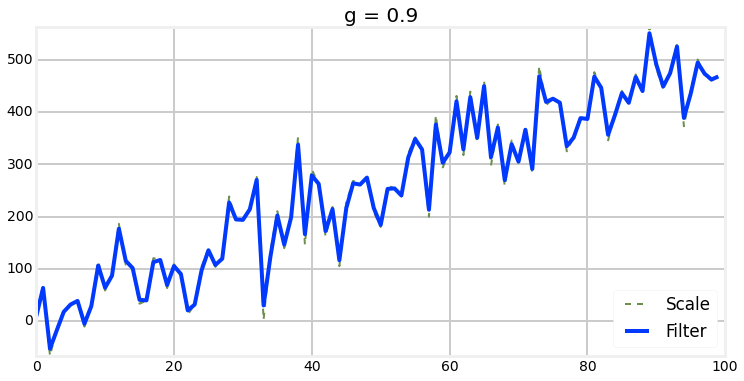
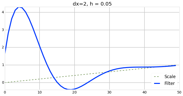
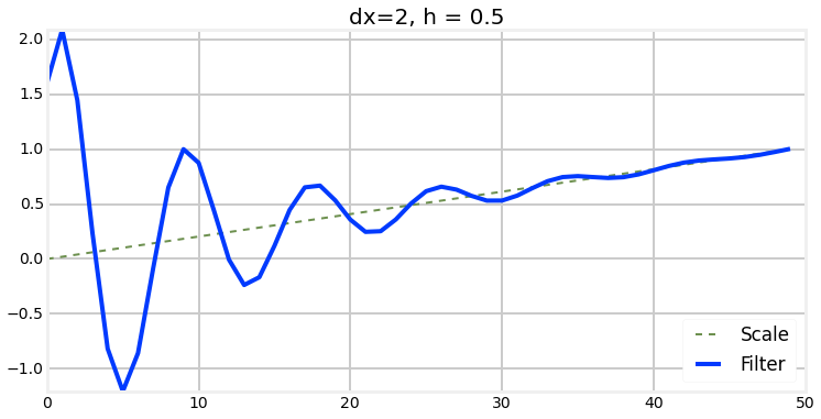
Choosing of H

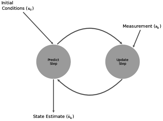
Kalman filter

Main idea

Assume imperfect sensor measurements.
We need Object motion model.
Our measurements contains measurement noise
Process noise describes imperfect object motion model

Kalman filter

How to describe measurement?

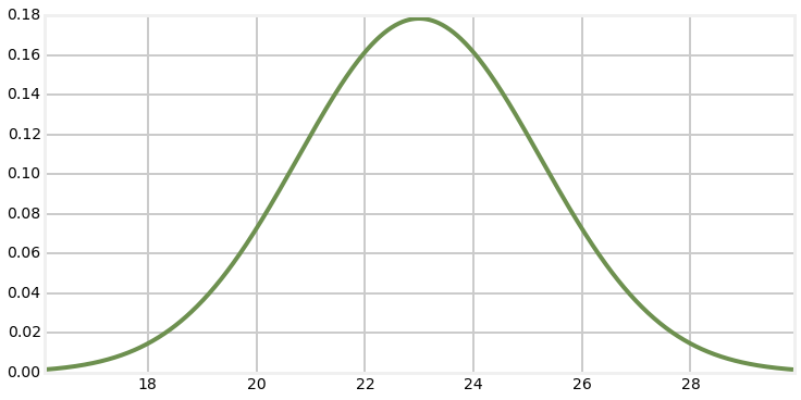
f(x,\mu,\sigma) = \frac{1}{{\sigma \sqrt {2\pi } }}e^{-\frac{(x - \mu)^2}{2 \sigma^2}}

f (x, μ, σ) = \frac{​ 1 ​ ​}{​ σ \sqrt ​ 2 π ​ ​ ​ ​} e ​ - \frac{​ ( x - μ ) ​ 2 ​ ​ ​ ​}{​ 2 σ ​ 2 ​ ​ ​} ​ ​

(\mu,\sigma^2)

(μ, σ ​ 2 ​ ​)

X ~ N

Kalman filter - 1D

Initial conditions

First expected values can be random
Describe confidence with big variance

N({\mu}_1, {{\sigma}_1}^2)+N({\mu}_2, {{\sigma}_2}^2) = N({\mu}_1 + {\mu}_2, {{\sigma}_1}^2 + {{\sigma}_2}^2)

N (μ ​ 1 ​ ​, σ ​ 1 ​ ​ ​ 2 ​ ​) + N (μ ​ 2 ​ ​, σ ​ 2 ​ ​ ​ 2 ​ ​) = N (μ ​ 1 ​ ​ + μ ​ 2 ​ ​, σ ​ 1 ​ ​ ​ 2 ​ ​ + σ ​ 2 ​ ​ ​ 2 ​ ​)

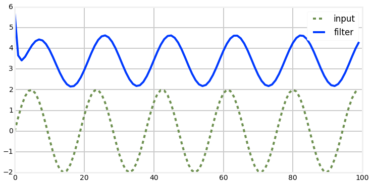
Prediction step

Sum of gaussians

Kalman filter - 1D

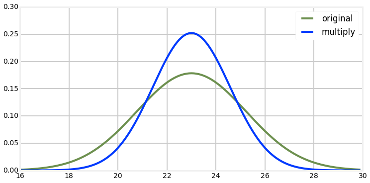
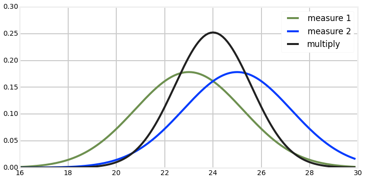
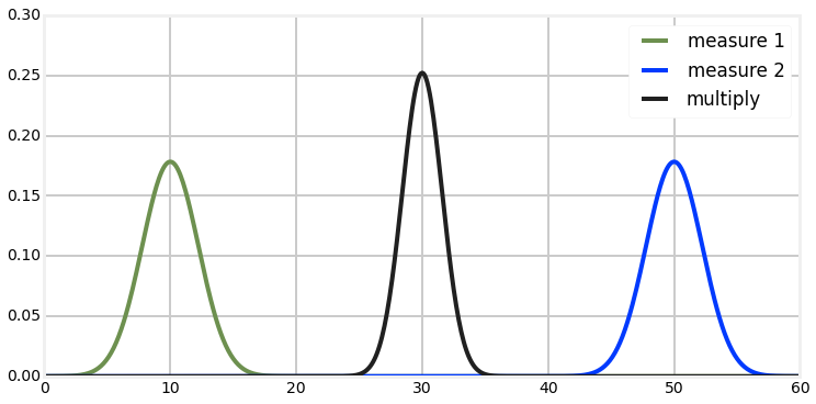
Correction step

Multiplication of gaussians

\mu=\frac{\sigma_1^2 \mu_2 + \sigma_2^2 \mu_1} {\sigma_1^2 + \sigma_2^2}

μ = \frac{​ σ ​ 1 ​ 2 ​ ​ μ ​ 2 ​ ​ + σ ​ 2 ​ 2 ​ ​ μ ​ 1 ​ ​ ​ ​}{​ σ ​ 1 ​ 2 ​ ​ + σ ​ 2 ​ 2 ​ ​ ​}

\sigma^2 = \frac{1}{\frac{1}{\sigma_1^2} + \frac{1}{\sigma_2^2}}

σ ​ 2 ​ ​ = \frac{​ 1 ​ ​}{​ \frac{​ 1 ​ ​}{​ σ ​ 1 ​ 2 ​ ​ ​} + \frac{​ 1 ​ ​}{​ σ ​ 2 ​ 2 ​ ​ ​} ​}

Kalman filter - 1D

Example for understanding

Kalman filter - 1D

Relationship to G-H filter

g_n = \frac{\sigma^2_{x'}}{\sigma^2_{y}}

g ​ n ​ ​ = \frac{​ σ ​ x ​ ' ​ ​ ​ 2 ​ ​ ​ ​}{​ σ ​ y ​ 2 ​ ​ ​}

h_n = \frac{COV (x,\dot{x})}{\sigma^2_{y}}

h ​ n ​ ​ = \frac{​ C O V ( x , ​ x ​ ˙ ​ ​ ) ​ ​}{​ σ ​ y ​ 2 ​ ​ ​}

\mu_{x'}=\frac{\sigma_1^2 \mu_2 + \sigma_2^2 \mu_1} {\sigma_1^2 + \sigma_2^2} = \frac{ya + xb} {a+b}

μ ​ x ​' ​ ​ ​ ​ = \frac{​ σ ​ 1 ​ 2 ​ ​ μ ​ 2 ​ ​ + σ ​ 2 ​ 2 ​ ​ μ ​ 1 ​ ​ ​ ​}{​ σ ​ 1 ​ 2 ​ ​ + σ ​ 2 ​ 2 ​ ​ ​} = \frac{​ y a + x b ​ ​}{​ a + b ​}

{\sigma_{x'}^2} = \frac{1}{ \frac{1}{\sigma_1^2} + \frac{1}{\sigma_2^2}} = \frac{1}{ \frac{1}{a} + \frac{1}{b}}

σ ​ x ​' ​ ​ ​ 2 ​ ​ = \frac{​ 1 ​ ​}{​ \frac{​ 1 ​ ​}{​ σ ​ 1 ​ 2 ​ ​ ​} + \frac{​ 1 ​ ​}{​ σ ​ 2 ​ 2 ​ ​ ​} ​} = \frac{​ 1 ​ ​}{​ \frac{​ 1 ​ ​}{​ a ​} + \frac{​ 1 ​ ​}{​ b ​} ​}

Kalman filter - 1D

Extreme amount of noise

Kalman filter - 1D

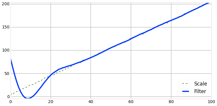
Bad Initial Estimate

Kalman filter - 1D

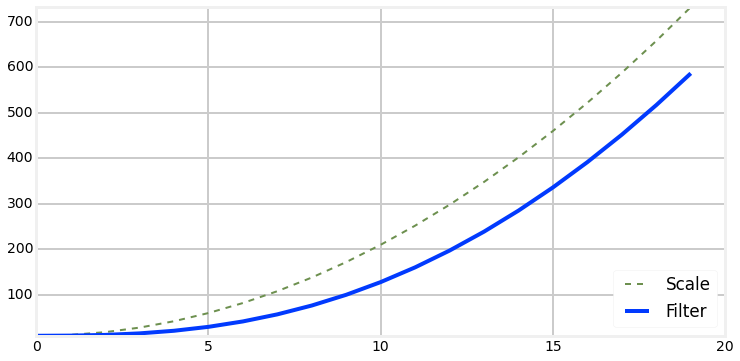
Nonlinear Systems

Terrible!

Kalman filter - 1D

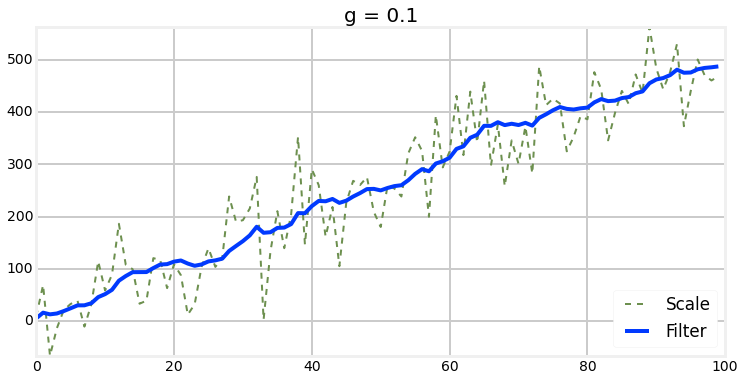
Noisy Nonlinear Systems

Terrible!

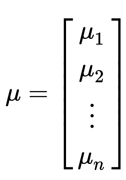
Multivariate Kalman filter

What is different?

N(\mu,\,\Sigma) = (2\pi)^{-\frac{n}{2}}|\Sigma|^{-\frac{1}{2}}\, e^{ -\frac{1}{2}(x-\mu)^T\Sigma^{-1}(x-\mu) }

N (μ, Σ) = (2 π) ​ - \frac{​ n ​ ​}{​ 2 ​} ​ ​ ∣ Σ ∣ ​ - \frac{​ 1 ​ ​}{​ 2 ​} ​ ​ e ​ - \frac{​ 1 ​ ​}{​ 2 ​} (x - μ) ​ T ​ ​ Σ ​ - 1 ​ ​ (x - μ) ​ ​

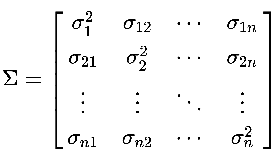
Multivariate Kalman filter

What is different?

Multivariate Kalman filter

The superposition of the two covariances is where all the magic happens.

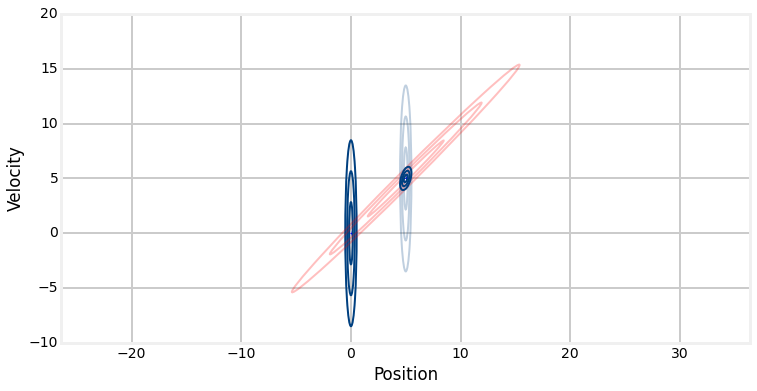
Velocity is unobserved variable

Multivariate Kalman filter

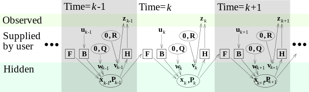
Algorithm

Prediction step

x^- = F x + B u

x ​ - ​ ​ = F x + B u

P^- = {FP{F}}^T + Q

P ​ - ​ ​ = F P F ​ T ​ ​ + Q

Update step

y = z - H x^-

y = z - H x ​ - ​ ​

S = {HP^-H}^T + R

S = H P ​ - ​ ​ H ​ T ​ ​ + R

K = {P^-H}^T {S}^{-1}

K = P ​ - ​ ​ H ​ T ​ ​ S ​ - 1 ​ ​

x = x^- Ky

x = x ​ - ​ ​ K y

P = (I-KH)P^-

P = (I - K H) P ​ - ​ ​

Legend

x - state
P - uncertainty covariance
Q - process uncertainty
u - motion vector
B - control transition matrix
F - state transition matrix
H - measurement function
R - state uncertainty
S - measurement space
K - kalman gain

Multivariate Kalman filter

Algorithm

Prediction step

x^- = F x + B u

x^- = F x + B u

P^- = {FP{F}}^T + Q

P^- = {FP{F}}^T + Q

Update step

y = z - H x^-

y = z - H x^-

S = {HP^-H}^T + R

S = {HP^-H}^T + R

K = {P^-H}^T {S}^{-1}

K = {P^-H}^T {S}^{-1}

x = x^- Ky

x = x^- Ky

P = (I-KH)P^-

P = (I-KH)P^-

Innovation or measurement residual

Innovation (or residual) covariance

Map system uncertainty into optimal kalman gain

Updated (a posteriori) state estimate

Predicted (a priori) state estimate

Predicted (a priori) estimate covariance

Updated (a posteriori) estimate covariance

Multivariate Kalman filter

Algorithm

predict the next value for x
adjust covariance for x for uncertainty caused by prediction
get measurement for x
compute residual as: "x - x_prediction"
compute kalman gain based on noise levels
compute new position as "residual * kalman gain"
compute covariance for x to account for additional information the measurement provides

Multivariate Kalman filter

Algorithm

Kalman filter - step by step

1. Initialization

initialize state x and covariance matrix P

2. Design transition function

encode object motion model to transition function matrix
e.g.:

x^- = \dot{x}\Delta t + x

x^- = \dot{x}\Delta t + x

3. Design the Motion Function

Design control input and state function
Optional (u = 0)

Kalman filter - step by step

4. Design the Measurement Function

Design measurement function in matrix form
Residual need to be from same measurement space, otherwise it's nonsense

5. Design the Measurement Noise Matrix

The measurement noise matrix models the noise of sensors as a covariance matrix.
e.g. White noise

6. Design the Process Noise Matrix

quite demanging, out of scope this presentation

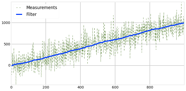
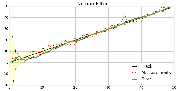
Plots

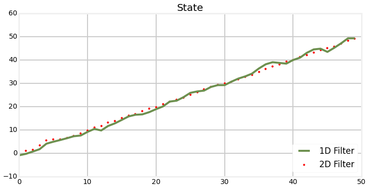
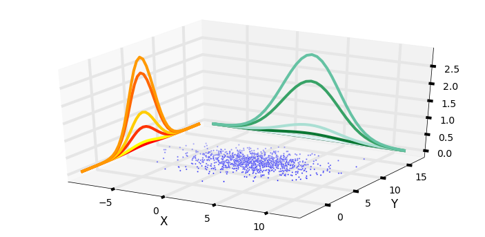
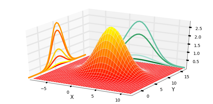
1D vs 2D

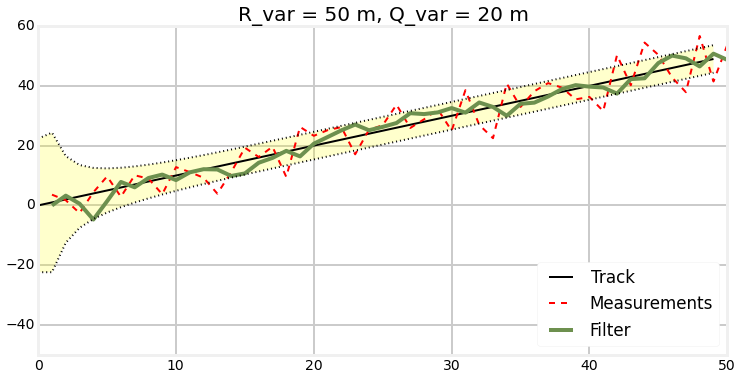
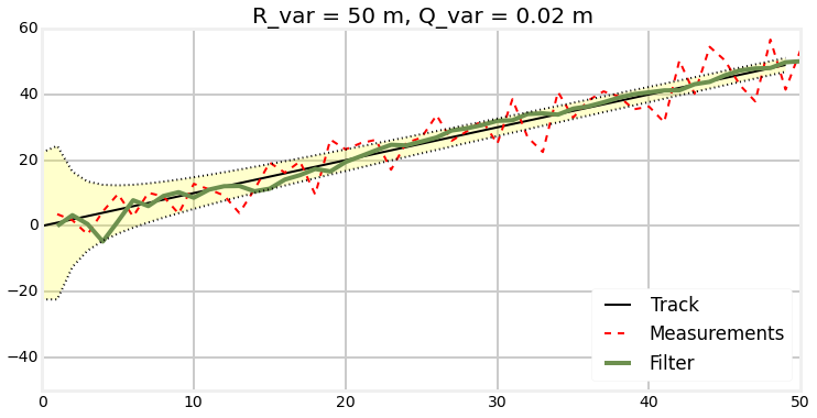
Plots

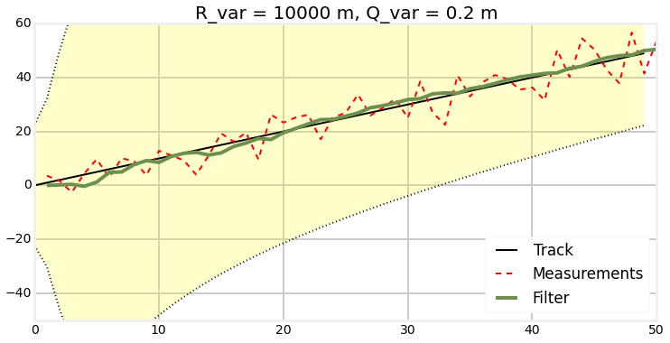
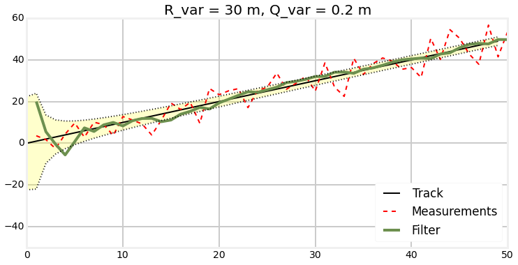
Process noise

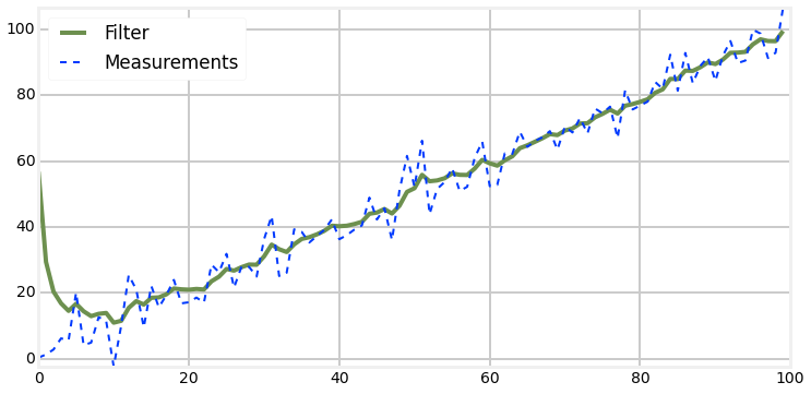
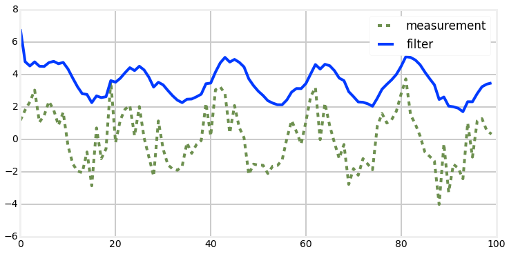
Plots

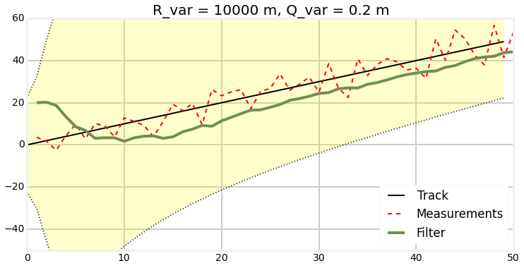
Measurement noise and bad init

Plots

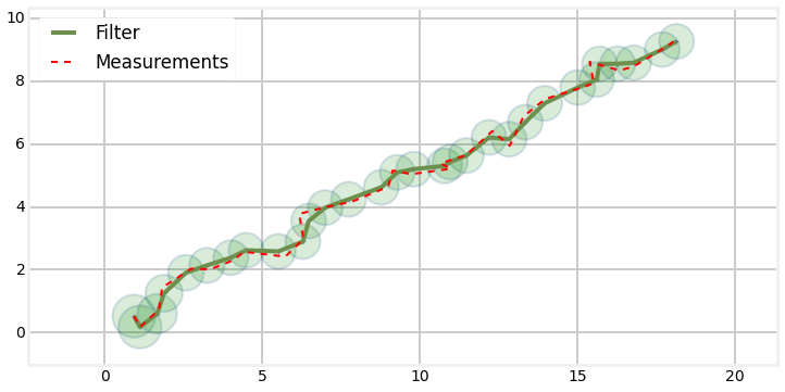
Progress

Plots

Animated progress

Related filters

Extended Kalman filter - solves problem of the nonlinear model

Unscented Kalman filter - better than EKF if the model is highly nonlinear

Kalman–Bucy filter - continuous time version of the Kalman filter

Hybrid Kalman filter - continuous-time models, discrete-time measurements

Summary

Disadvantages:

Nonlinear models
Initialization
Discrete time

Advantages:

Disadvantages can be solved by related filters. E.g.: Extended Kalman filter, Unscented Kalman filter ....
The process noise or the measurement noise can be described in some specific problems
Its recursive structure allows its real-time execution without storing observations or past estimates.
Can be used in multidimensional space

Applications

Attitude and Heading Reference Systems
Autopilot
Battery state of charge (SoC) estimation[40][41]
Brain-computer interface
Chaotic signals
Tracking and Vertex Fitting of charged particles inParticle Detectors [42]
Tracking of objects in computer vision
Dynamic positioning
Economics, in particular macroeconomics, time series analysis, and econometrics [43]
Inertial guidance system
Orbit Determination
Power system state estimation
Radar tracker
Satellite navigation systems
Seismology [44]
Sensorless control of AC motor variable-frequency drives
Simultaneous localization and mapping
Speech enhancement
Visual odometry
Weather forecasting
Navigation system
3D modeling
Structural health monitoring
Human sensorimotor processing [45]

Attitude and Heading Reference Systems
Autopilot
Battery state of charge estimation
Tracking of objects in computer vision
Dynamic positioning
Economics
Inertial guidance system
Orbit Determination
Power system state estimation

Radar tracker
Satellite navigation systems
Seismology
Simultaneous localization and mapping
Speech enhancement
Visual odometry
Weather forecasting
Navigation system
Structural health monitoring
Human sensorimotor processing

Applications

Adaptive Kalman Filter - Navigation signal lost in tunnel

Object tracking - OpenCV

References

Visual object tracking

2D Kalman tracking

JURIĆ, Darko. Code of practice for project management for construction and development. Code Project [online]. [cit. 2015-03-28]. Dostupné z: http://www.codeproject.com/Articles/865935/Object-Tracking-Kalman-Filter-with-Ease

Kalman Filters and Random Signals in Python. LABBE, Roger. [online]. [cit. 2015-03-28]. Dostupné z: http://nbviewer.ipython.org/github/rlabbe/Kalman-and-Bayesian-Filters-in-Python/blob/master/table_of_contents.ipynb
Kalman filter. In: Wikipedia: the free encyclopedia [online]. San Francisco (CA): Wikimedia Foundation, 2001- [cit. 2015-03-29]. Dostupné z: http://en.wikipedia.org/wiki/Kalman_filter

Kalman filter

History

G-H Filter

G-H Filter

G-H Filter

Bad initial condition

Acceleration

Choosing of G

Choosing of H

Kalman filter

Main idea

Kalman filter

Kalman filter - 1D

Initial conditions

Prediction step

Kalman filter - 1D

Correction step

Kalman filter - 1D

Kalman filter - 1D

Kalman filter - 1D

Relationship to G-H filter

Kalman filter - 1D

Kalman filter - 1D

Kalman filter - 1D

Extreme amount of noise

Kalman filter - 1D

Bad Initial Estimate

Kalman filter - 1D

Nonlinear Systems

Kalman filter - 1D

Noisy Nonlinear Systems

Multivariate Kalman filter

Multivariate Kalman filter

Multivariate Kalman filter

Multivariate Kalman filter

Algorithm

Multivariate Kalman filter

Algorithm

Multivariate Kalman filter

Algorithm

Multivariate Kalman filter

Algorithm

Kalman filter - step by step

1. Initialization

2. Design transition function

3. Design the Motion Function

Kalman filter - step by step

4. Design the Measurement Function

5. Design the Measurement Noise Matrix

6. Design the Process Noise Matrix

Plots

Plots

Plots

Plots

Plots

Plots

Related filters

Summary

Applications

Applications

Adaptive Kalman Filter - Navigation signal lost in tunnel

References

deck

More from Tomáš Šabata