Self-Driving Cars with Python

TOMASZ KACMAJOR


Trójmiasto
May 25, 2017
Image source: http://www.autonomous-car.com/2015/12/when-will-self-driving-cars-be-ready.html
TOMASZ KACMAJOR


www.tomaszkacmajor.pl
tomasz.kacmajor@gmail.com

AGENDA
LANE LINES FINDING
TRAFFIC SIGN CLASSIFICATION
BEHAVIORAL CLONING
MOTIVATION
THE INDUSTRY
SUMMARY Q&A
LANE LINES FINDING
TRAFFIC SIGN CLASSIFICATION
BEHAVIORAL CLONING
MOTIVATION
MOTIVATION

Self-Driving Car Nanodegree Program
Computer Vision
Deep Learning
Sensor Fusion
Localization
Control
Path Planning
Hiring Partners
Term 1
Term 2
Term 3
MOTIVATION
COMMUNITY
https://pythonprogramming.net/more-interesting-self-driving-python-plays-gta-v/
https://zhengludwig.wordpress.com/projects/self-driving-rc-car/
https://www.youtube.com/watch?v=asQ3vHOwHxw
https://www.youtube.com/watch?v=6oEQXnqpEGc
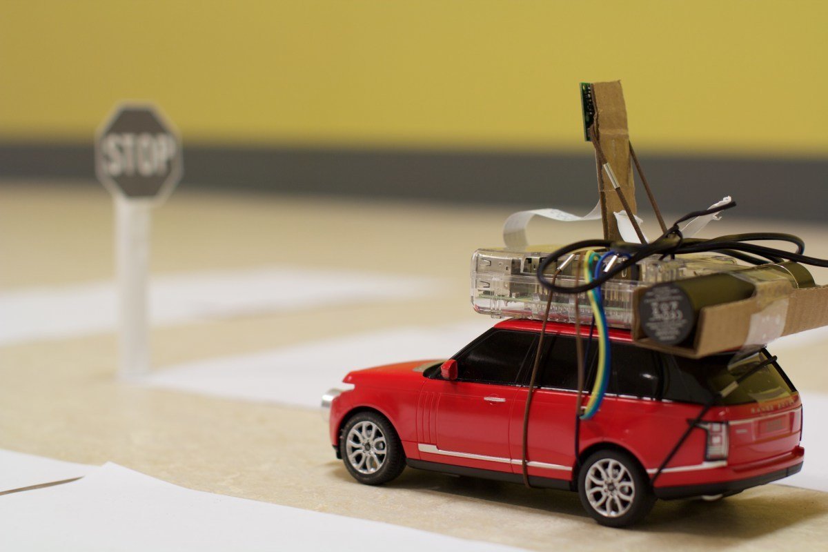
Self-Driving RC Car
Python plays GTA V
Autonomous RC car
Udacity/Didi SDC Challenge 2017
Arduino/Raspberry Pi projects
Simulators in games
Autonomous RC cars
Public challenges
THE INDUSTRY
HISTORY

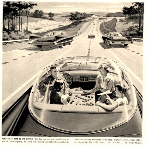
A Boy's Life Magazine, 1956
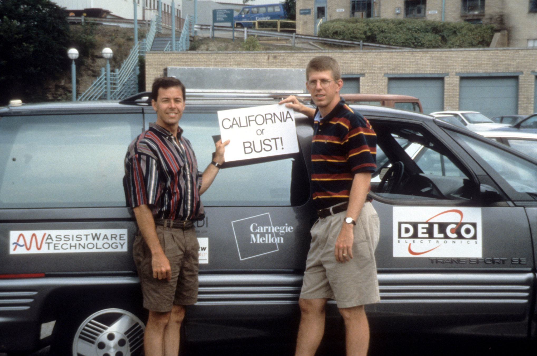
No Hands Across America, 1995
from: https://www.cs.cmu.edu/news/look-ma-no-hands-cmu-vehicle-steered-itself-across-country-20-years-ago
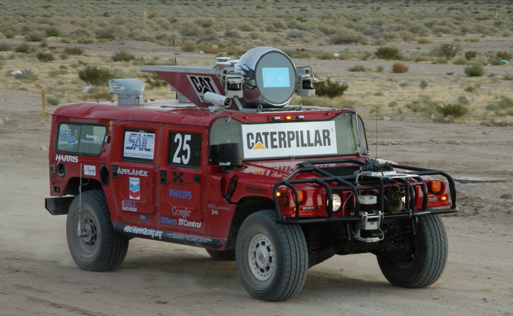
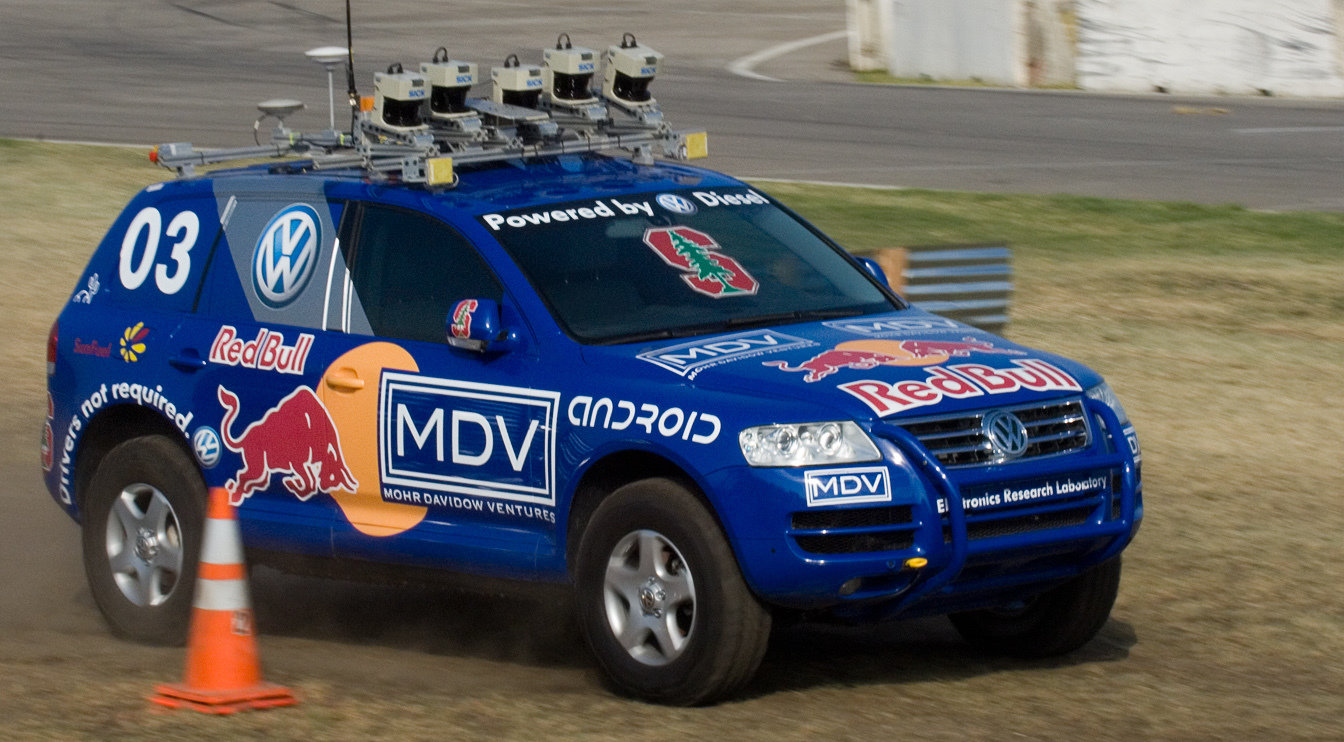
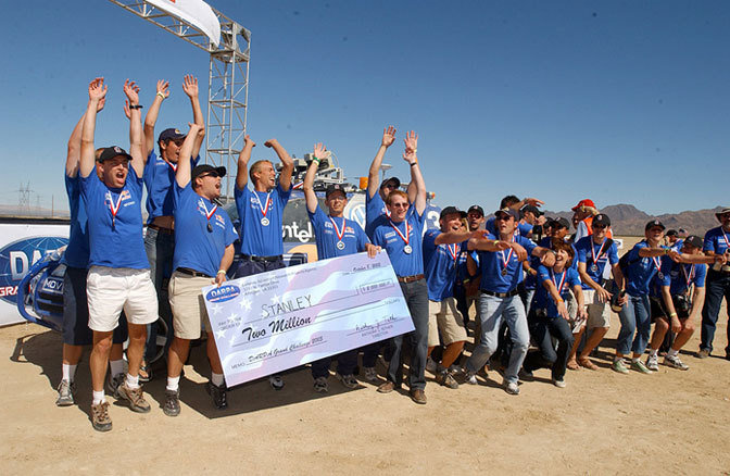
DARPA Grand Challenge, 2005
from: http://www.extremetech.com/extreme/115131-learn-how-to-program-a-self-driving-car-stanfords-ai-guru-says-he-can-teach-you-in-seven-weeks
DARPA Grand Challenge, 2005
http://www.pbs.org/wgbh/nova/tech/cars-drive-themselves.html
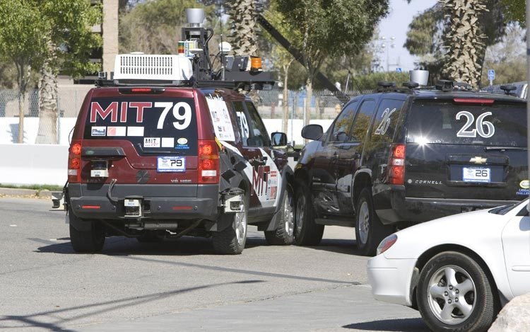
DARPA Urban Challenge, 2007
http://www.motortrend.com/news/darpa-urban-challenge-reflections/
DARPA Grand Challenge, 2004
from: http://www.cs.cmu.edu/~curmson/urmsonRobots.html
2009


comma.ai
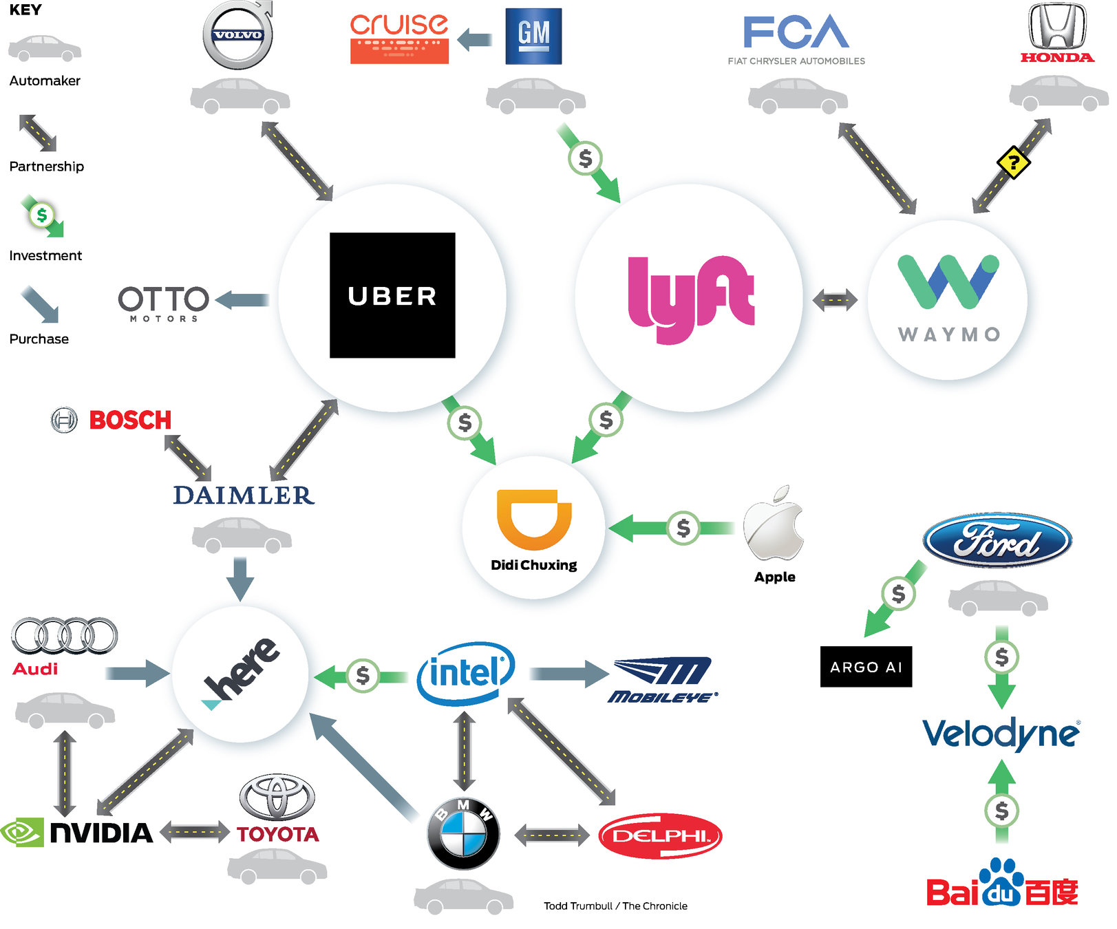
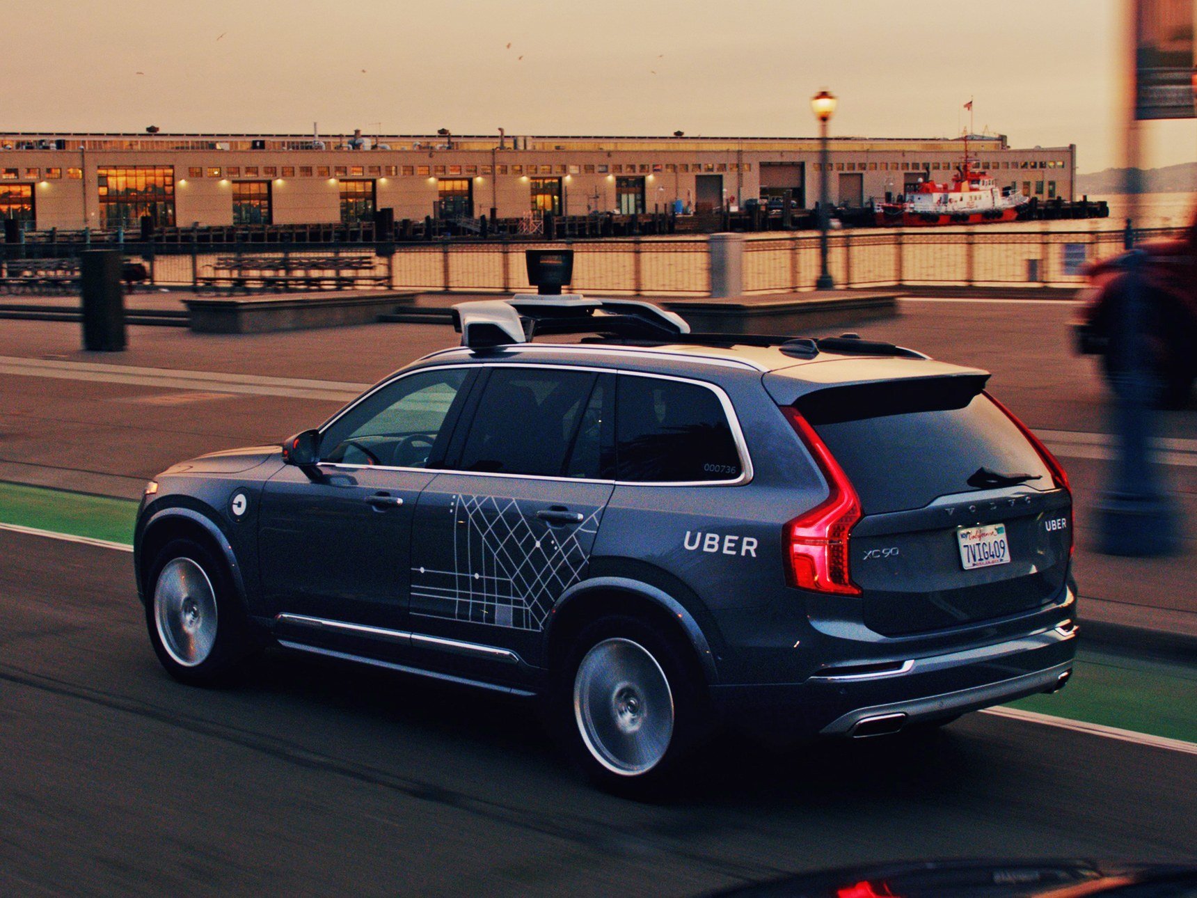
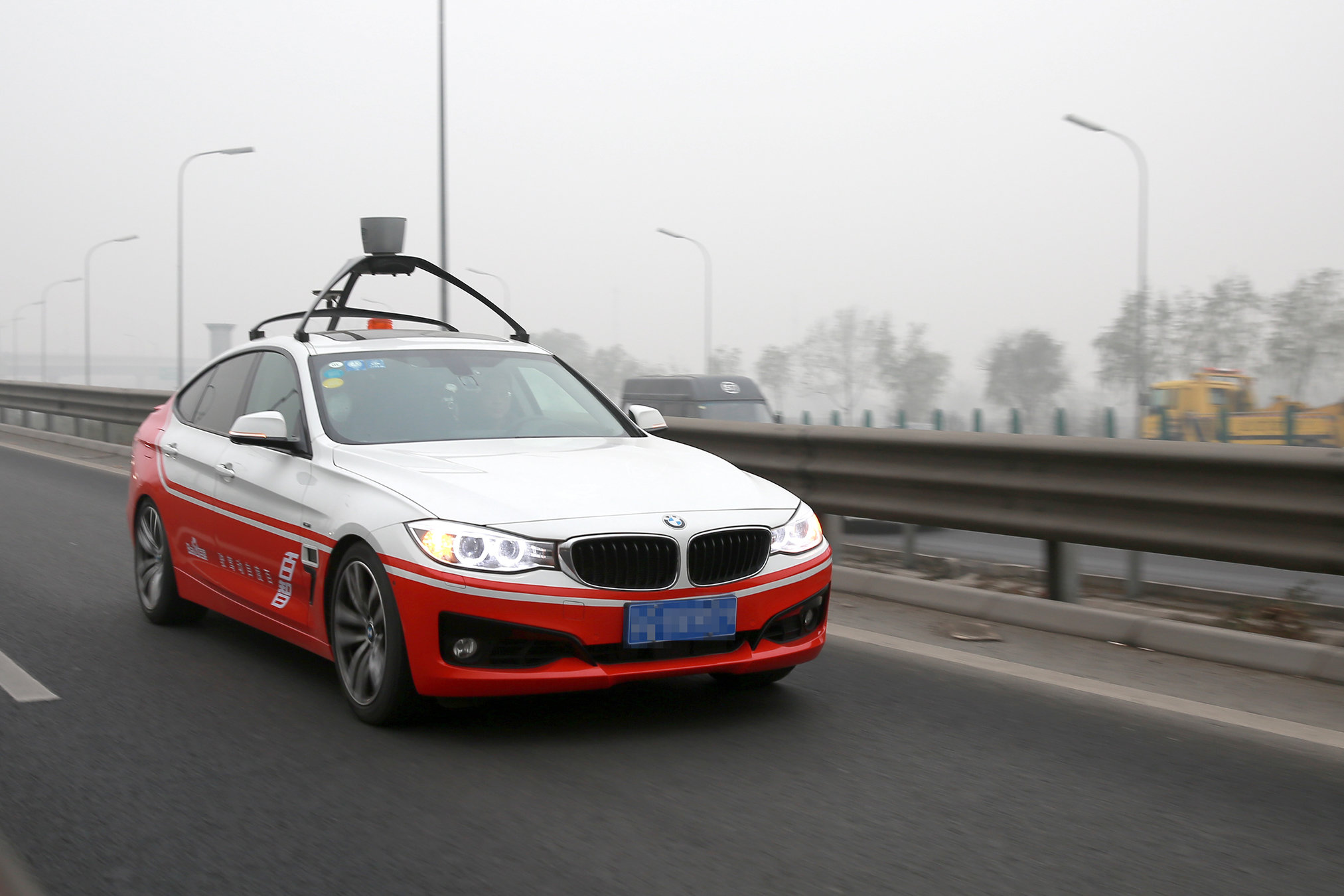
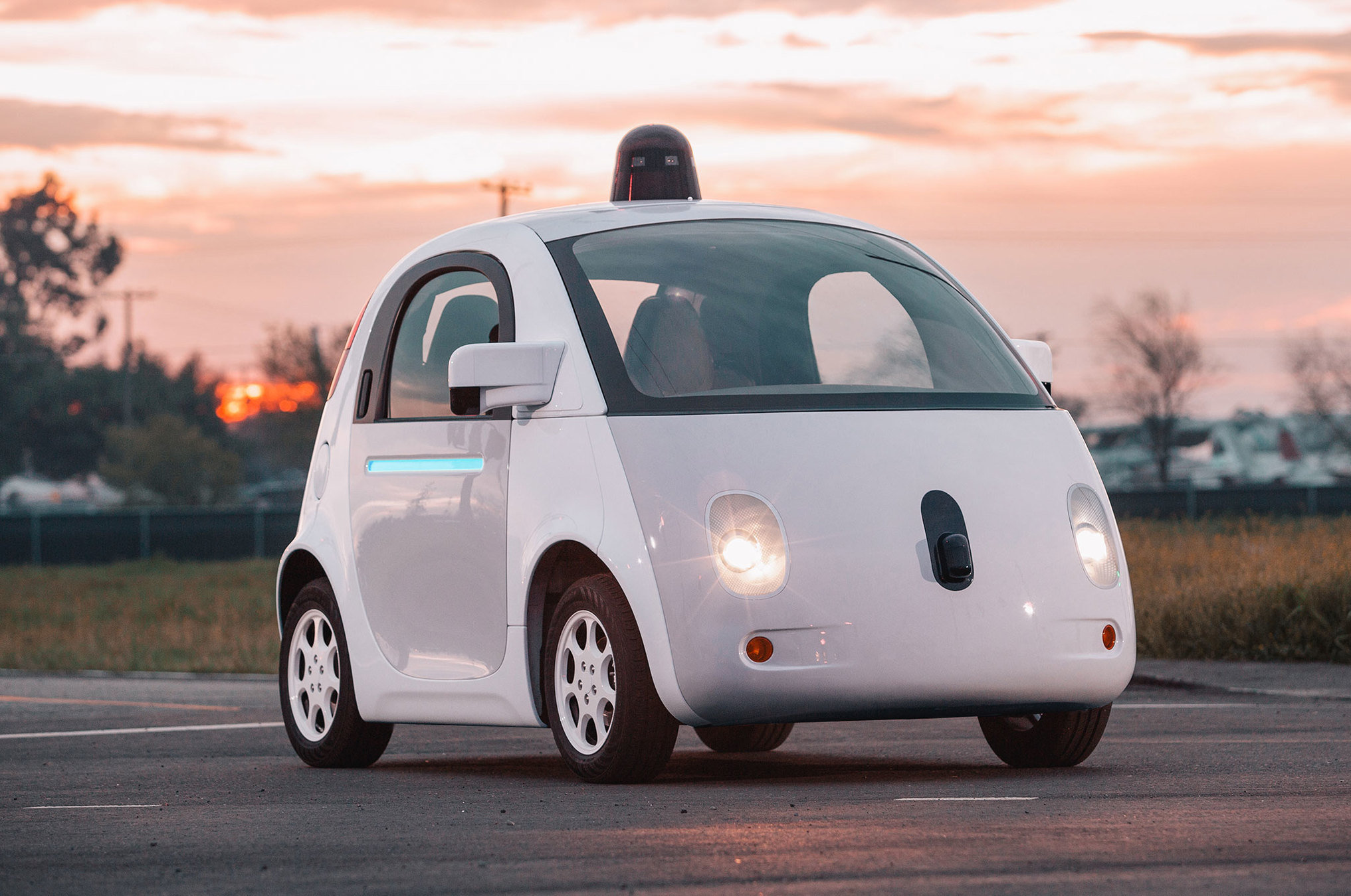
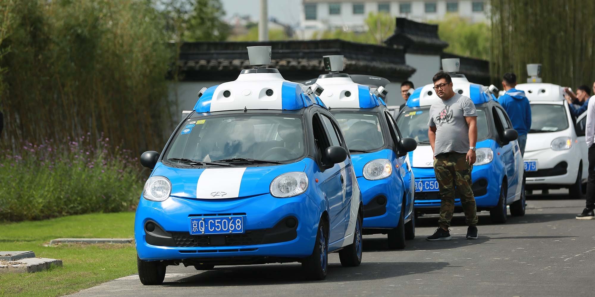
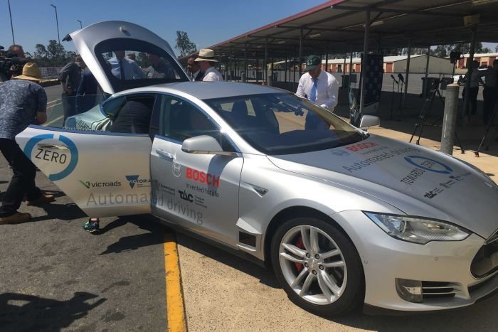
SELF-DRIVING CARS INDUSTRY
from: http://www.sfchronicle.com/business/article/Partner-up-Self-driving-car-firms-form-tangled-11160522.php
SELF-DRIVING
CARS INDUSTRY
THE INDUSTRY
PURPOSE - SAFETY
Car accidents in Poland
3000 deaths/year
8 deaths/day
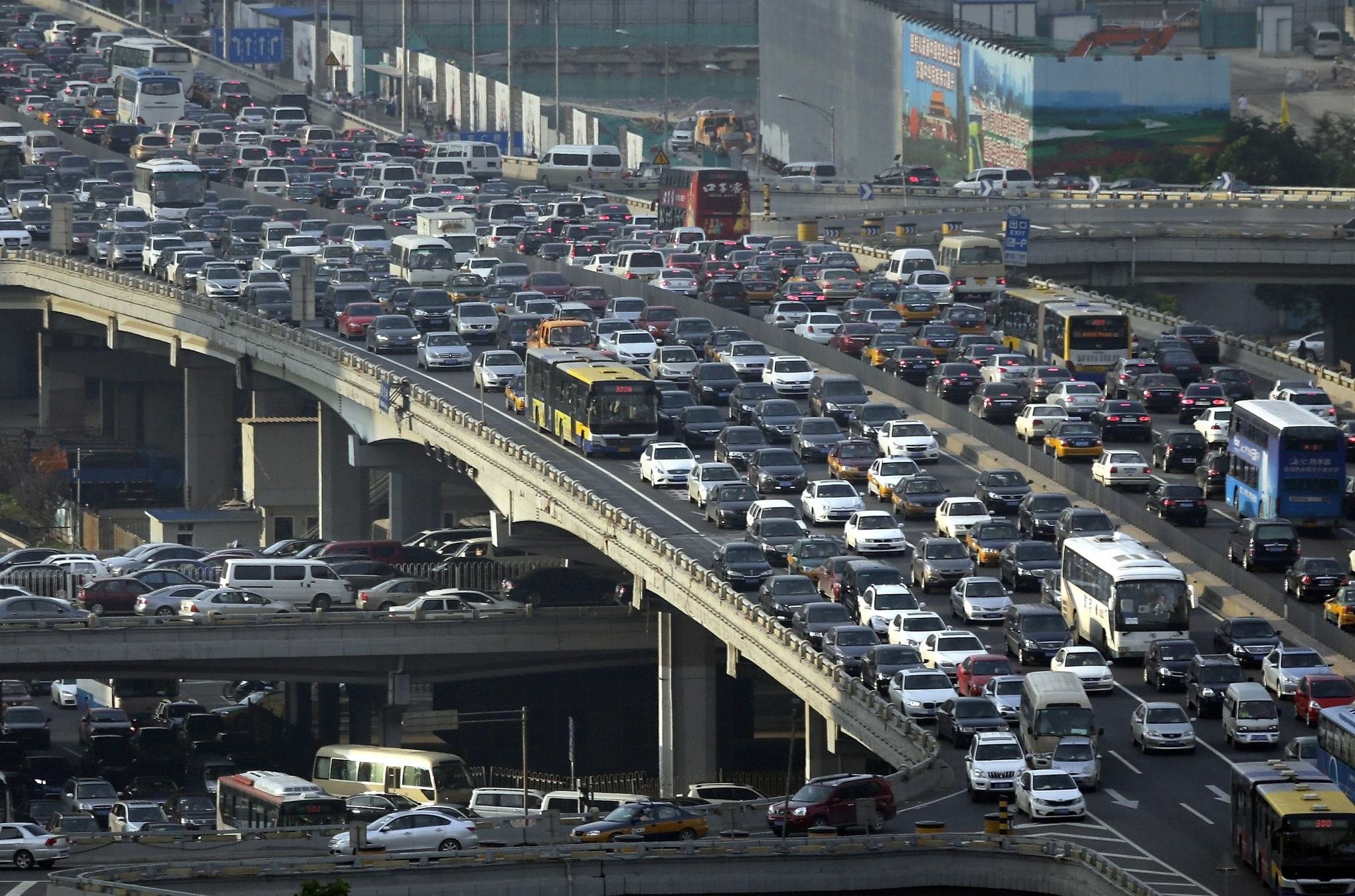
Growing congestion
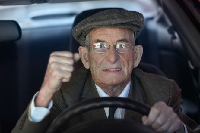
Helping elder or disabled people
THE INDUSTRY
COMPLEXITY
Artificial Ingelligence
Programming
Mechanics
Sensors
Localization
Radars
LIDARs
Cameras
Python
C++
HD Maps
GPS
Computing
Deep Neural Networks
Computer Vision
Cloud
GPU
Cyber-security
Sociology
Data centers
C
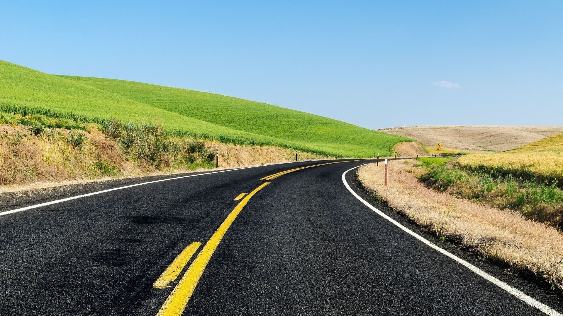
LANE LINES
FINDING


ver. 3.5.2
ver. 3.1.0
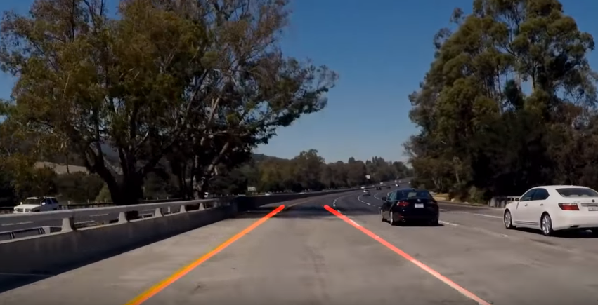
LANE LINES FINDING
PIPELINE
Reading image or video frame
Filtering white and yellow colors
Conversion to grayscale
Gaussian blurring
Edge detection
Region of interest definition
Hough lines detection
Filtering Hough lines
Averaging line segments
Applying moving average
on final lines
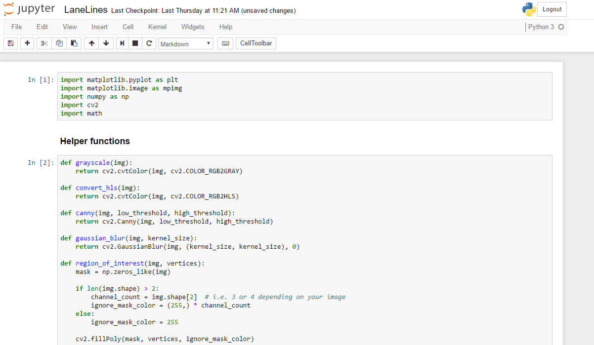
import matplotlib.pyplot as plt
import matplotlib.image as mpimg
import numpy as np
import cv2
import math
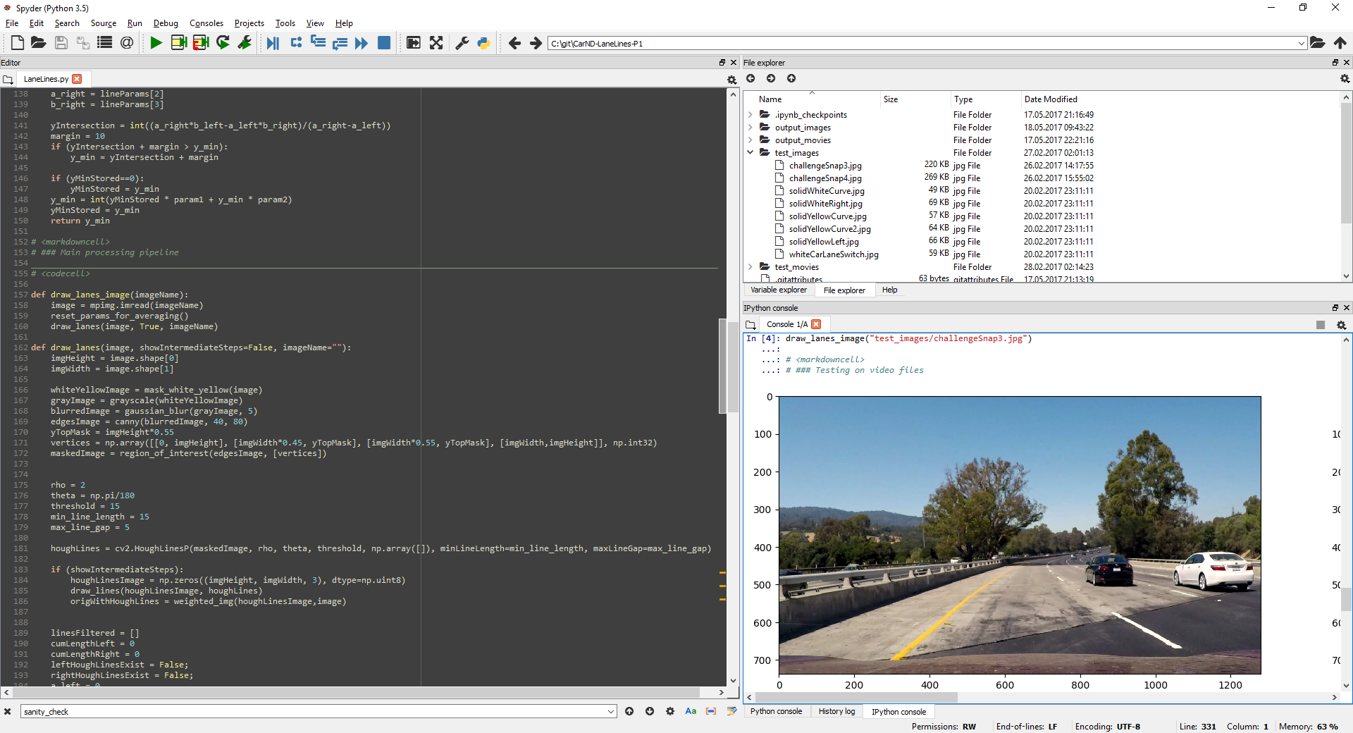
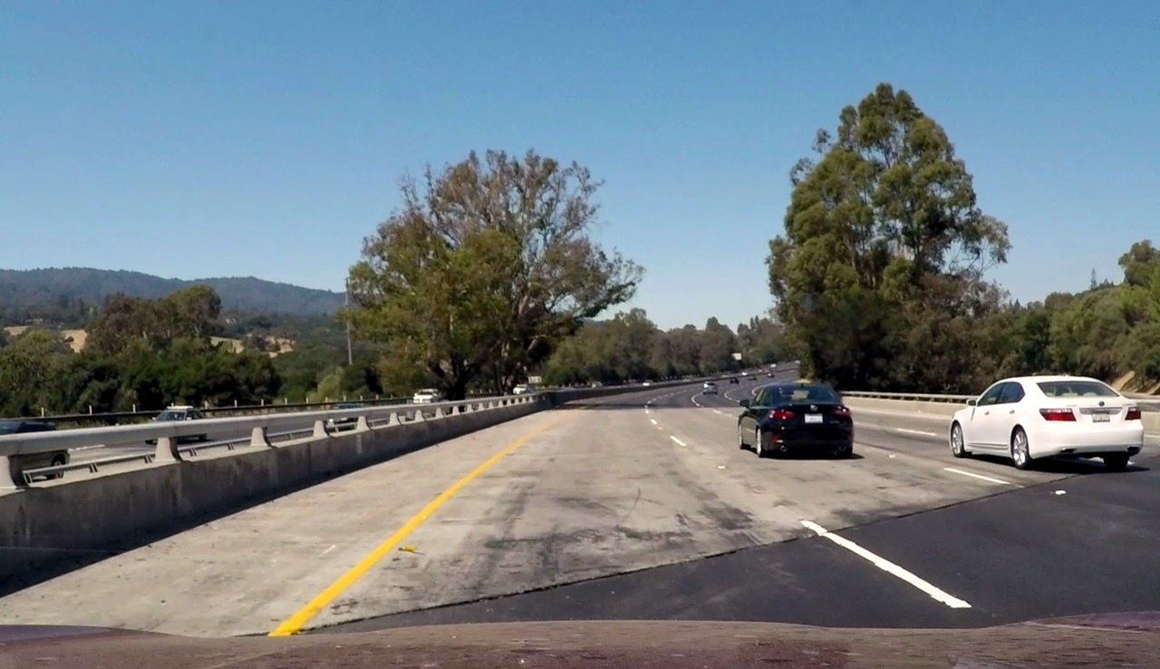
image_name = "test_images/challengeSnap3.jpg"
image = mpimg.imread(image_name)
#image = cv2.imread(image_name)
plt.imshow(image)
plt.show()LANE LINES FINDING
IMPLEMENTATION
Reading image
    image_gray = cv2.cvtColor(image, cv2.COLOR_BGR2GRAY)
    image_blurred = cv2.GaussianBlur(image_gray, (5, 5), 0)
    image_edges = cv2.Canny(image_blurred, 40, 80)

    plt.imshow(image_edges, cmap='gray')
    plt.show()
LANE LINES FINDING
IMPLEMENTATION
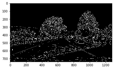
Edge detection - first approach
    h_channel = image[:,:,0]
    l_channel = image[:,:,1]
    s_channel = image[:,:,2]

    f, (ax1, ax2, ax3) = plt.subplots(1, 3, figsize=(15, 10))
    ax1.imshow(h_channel, cmap='gray')
    ax1.set_title('R Channel', fontsize=15)
    ax2.imshow(l_channel, cmap='gray')
    ax2.set_title('G Channel', fontsize=15)
    ax3.imshow(s_channel, cmap='gray')
    ax3.set_title('B Channel', fontsize=15)
    plt.show()

    image_hls = cv2.cvtColor(image, cv2.COLOR_RGB2HLS)
    h_channel = image_hls[:,:,0]
    l_channel = image_hls[:,:,1]
    s_channel = image_hls[:,:,2]

    f, (ax1, ax2, ax3) = plt.subplots(1, 3, figsize=(15, 10))
    ax1.imshow(h_channel, cmap='gray')
    ax1.set_title('H Channel', fontsize=15)
    ax2.imshow(l_channel, cmap='gray')
    ax2.set_title('L Channel', fontsize=15)
    ax3.imshow(s_channel, cmap='gray')
    ax3.set_title('S Channel', fontsize=15)
    plt.show()
LANE LINES FINDING
IMPLEMENTATION
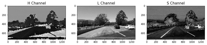
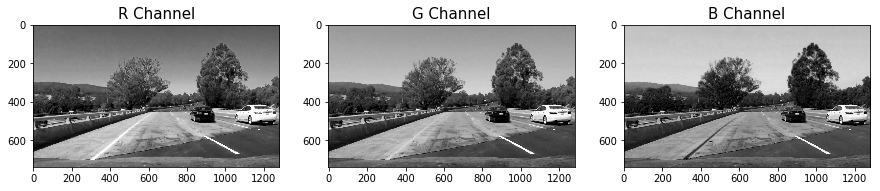
Different color spaces
    lower = np.uint8([  0, 200,   0])
    upper = np.uint8([255, 255, 255])
    white_mask = cv2.inRange(image_hls, lower, upper)

    lower = np.uint8([ 10,   0, 100])
    upper = np.uint8([ 40, 255, 255])
    yellow_mask = cv2.inRange(image_hls, lower, upper)

    mask = cv2.bitwise_or(white_mask, yellow_mask)
    masked_Image = cv2.bitwise_and(image, image, mask = mask)

    plt.imshow(masked_Image, cmap='gray')
    plt.show()
LANE LINES FINDING
IMPLEMENTATION
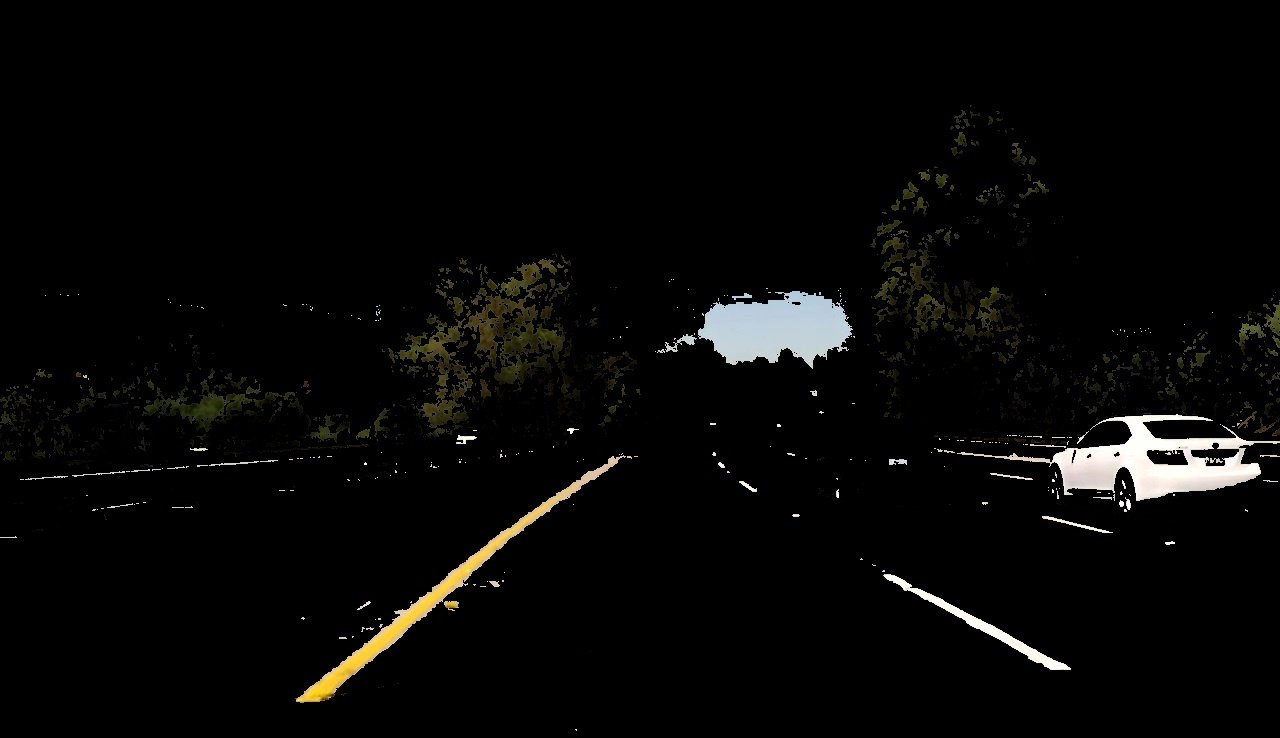
Filtering white and yellow colors
    image_gray = cv2.cvtColor(masked_Image, cv2.COLOR_BGR2GRAY)
    image_blurred = cv2.GaussianBlur(image_gray, (5, 5), 0)
    image_edges = cv2.Canny(image_blurred, 40, 80)

    fig = plt.figure(figsize = (30,20))
    plt.imshow(image_edges, cmap='gray')
    plt.show()
LANE LINES FINDING
IMPLEMENTATION
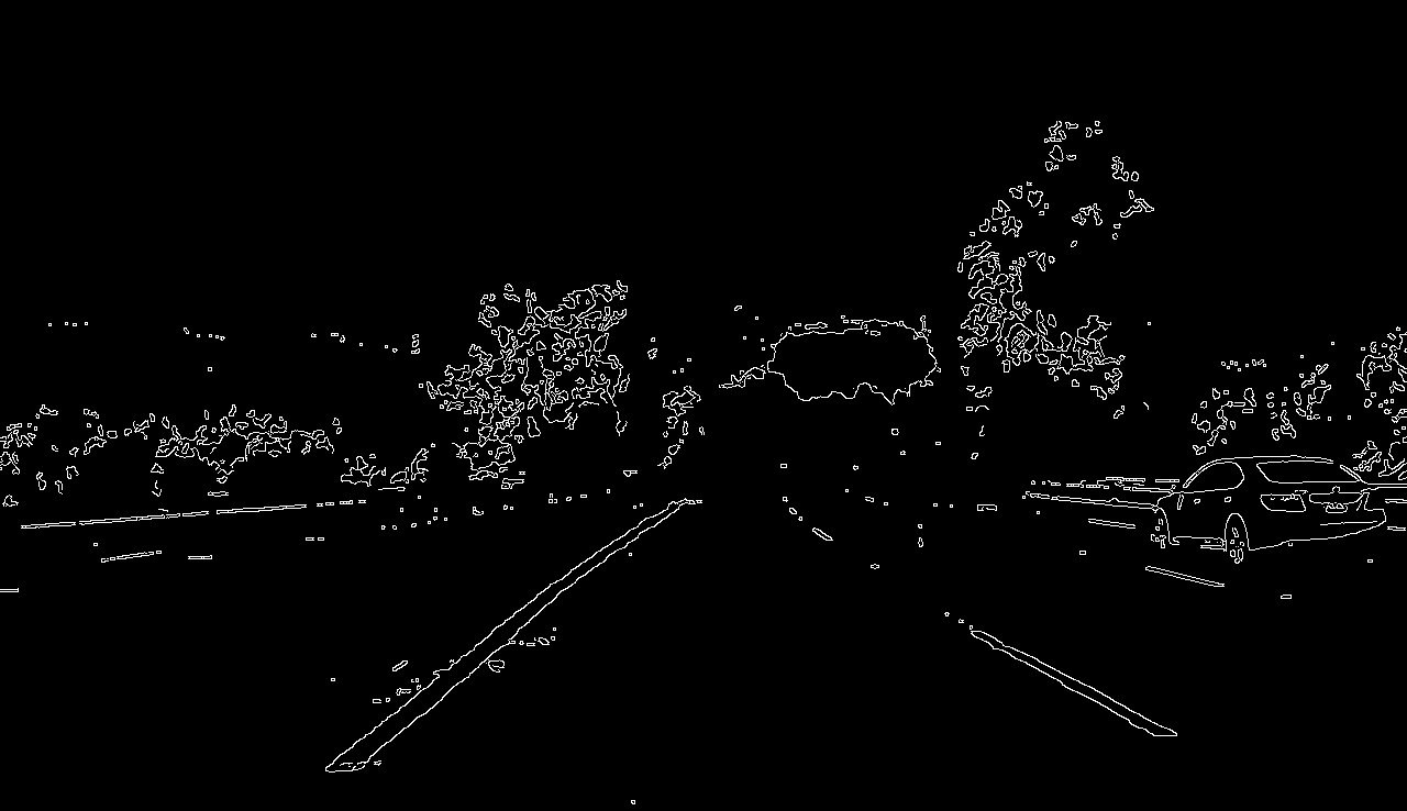
Edge detection
    imgHeight = image_edges.shape[0]
    imgWidth = image_edges.shape[1]
    yTopMask = imgHeight*0.55
    vertices = np.array([[0, imgHeight], [imgWidth*0.45, yTopMask], [imgWidth*0.55, yTopMask], [imgWidth,imgHeight]], np.int32)

    image_w_poly = np.copy(image_edges)
    cv2.polylines(image_w_poly, [vertices], True, color=(255,255,255), thickness=3)
    plt.imshow(image_w_poly, cmap='gray')
    plt.show()

    mask = np.zeros_like(image_edges)
    cv2.fillPoly(mask, [vertices], 255)
    masked_image = cv2.bitwise_and(image_edges, mask)

    fig = plt.figure(figsize = (30,20))
    plt.imshow(masked_image, cmap='gray')
    plt.show()
LANE LINES FINDING
IMPLEMENTATION
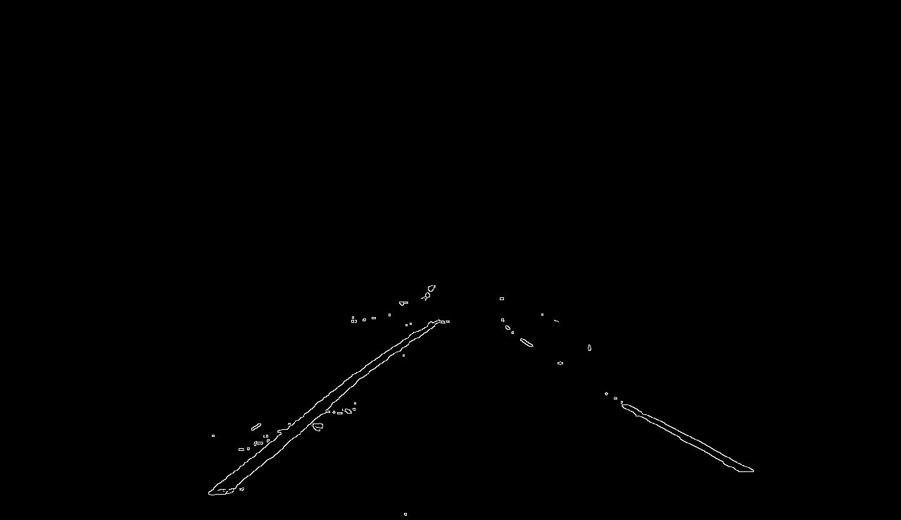
Region of interest definition
LANE LINES FINDING
IMPLEMENTATION
Hough lines detection
r
\theta
x
y
\theta
\rho
\rho = x cos(\theta) + y sin(\theta)

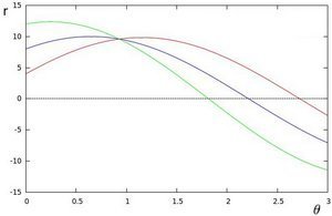
x
y

LANE LINES FINDING
IMPLEMENTATION
Hough lines detection
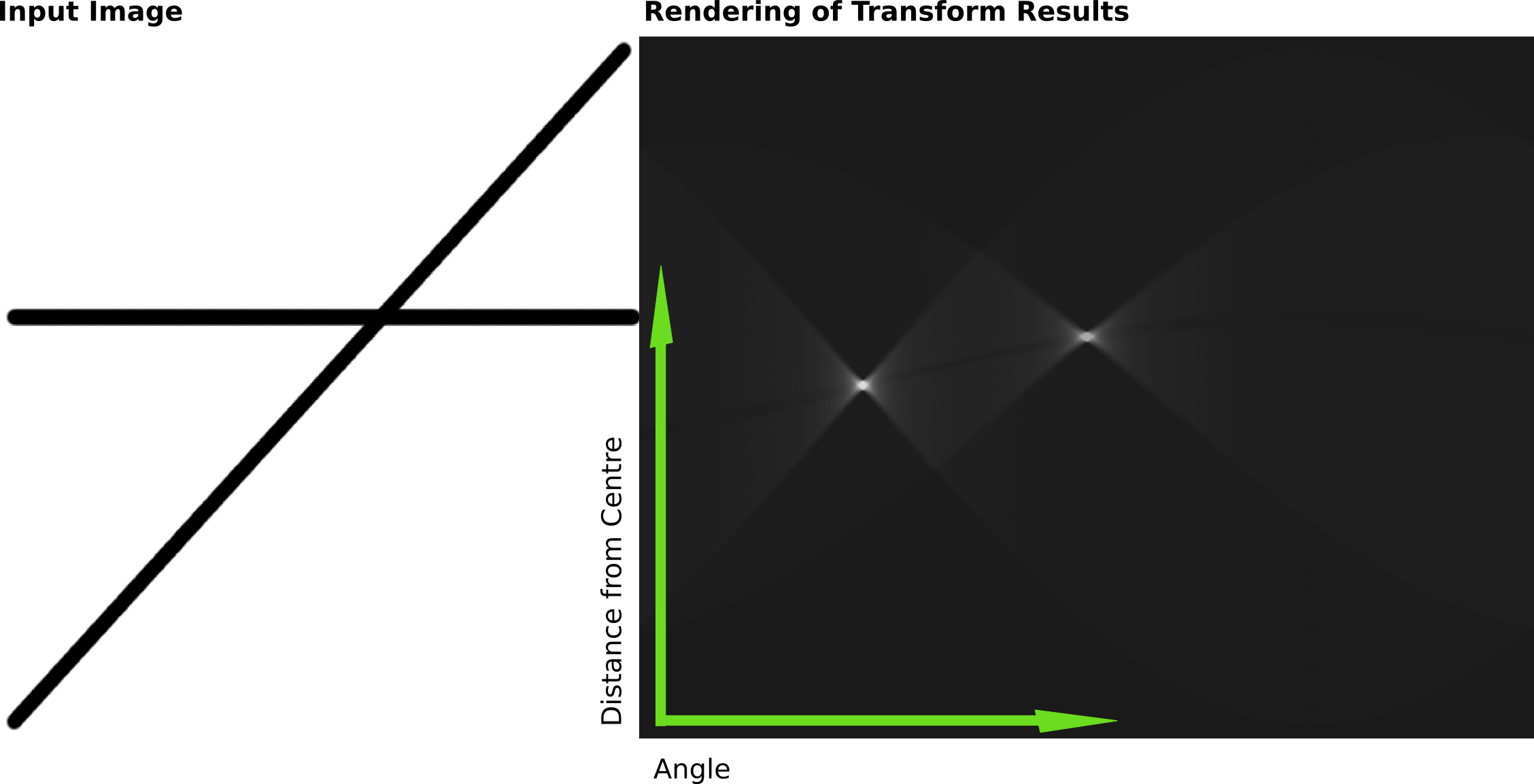
https://en.wikipedia.org/wiki/Hough_transform
LANE LINES FINDING
IMPLEMENTATION
Hough lines detection
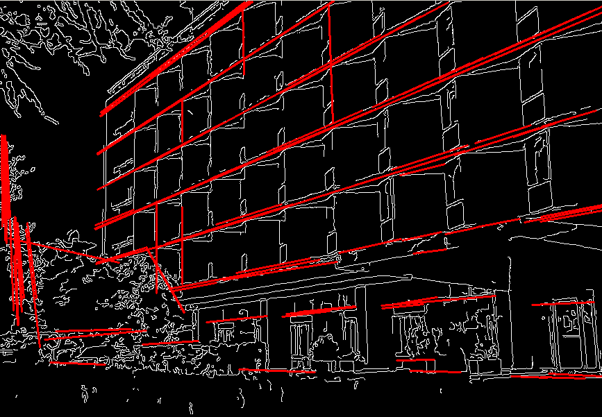
    rho = 2
    theta = np.pi/180
    threshold = 15
    min_line_length = 15
    max_line_gap = 5

    houghLines = cv2.HoughLinesP(masked_image, rho, theta, threshold, np.array([]), \
                                 minLineLength=min_line_length, maxLineGap=max_line_gap)

    houghLinesImage = np.zeros((imgHeight, imgWidth, 3), dtype=np.uint8)

    color=[0, 255, 0]
    thickness=2

    for line in houghLines:
        for x1,y1,x2,y2 in line:
            cv2.line(houghLinesImage, (x1, y1), (x2, y2), color, thickness)

    α=0.8
    β=1.0
    λ=0.0
    origWithHoughLines = cv2.addWeighted(image, α, houghLinesImage, β, λ)
    fig = plt.figure(figsize = (30,20))
    plt.imshow(origWithHoughLines)
    plt.show()
LANE LINES FINDING
IMPLEMENTATION
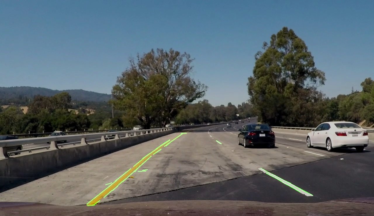
Hough lines detection
linesFiltered = []
for line in houghLines:
for x1,y1,x2,y2 in line:
if not np.isnan(a) or np.isinf(a) or (a == 0):
if (a > -1.5) and (a < -0.3) : # 0.3 corresponds to 17 degrees,
linesFiltered.append(line) # 1.5 corresponds to 56 degrees
if (a > 0.3) and (a < 1.5) :
linesFiltered.append(line)
houghLinesFilteredImage = np.zeros((imgHeight, imgWidth, 3), dtype=np.uint8)
for line in linesFiltered:
for x1,y1,x2,y2 in line:
cv2.line(houghLinesFilteredImage, (x1, y1), (x2, y2), \
color, thickness)
α=0.8
β=1.0
λ=0.0
origWithHoughLinesFiltered = cv2.addWeighted(image, α,\
houghLinesFilteredImage, β, λ)
fig = plt.figure(figsize = (30,20))
plt.imshow(origWithHoughLinesFiltered)
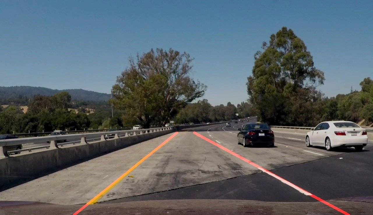
plt.show()LANE LINES FINDING
IMPLEMENTATION

Filtering Hough lines
LANE LINES FINDING
IMPLEMENTATION
a_{avg} = \frac{(a_{1}l_{1}^2 + a_{2}l_{2}^2 + ... + a_{n}l_{n}^2)}{l_{1}^2 + l_{2}^2 + ... + l_{n}^2}
a_{1}, l_{1}
a_{2}, l_{2}
a_{4}, l_{4}
a_{5}, l_{5}
a_{3}, l_{3}
a_{5}, l_{5}
a_{avg}
Averaging line segments
LANE LINES FINDING
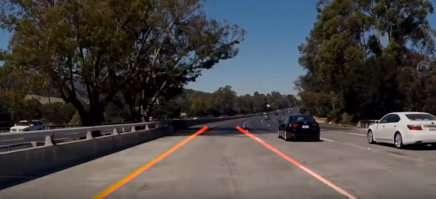
RESULTS
Sample of another, more complex
project in the course
My recording - Polish road
My recording - Polish road
TRAFFIC SIGN CLASSIFICATION


TRAFFIC SIGN CLASSIFICATION
Loading the data
Data exploration and visualization
Data preprocessing
Data augmentation
Designing, training and testing a CNN model
Using the model on new images
Analyzing softmax probabilities
IMPLEMENTATION
TRAFFIC SIGN CLASSIFICATION
import pickle
training_file = "./traffic-signs-data/train.p"
validation_file="./traffic-signs-data/valid.p"
testing_file = "./traffic-signs-data/test.p"
with open(training_file, mode='rb') as f:
train = pickle.load(f)
with open(validation_file, mode='rb') as f:
valid = pickle.load(f)
with open(testing_file, mode='rb') as f:
test = pickle.load(f)
X_train, y_train = train['features'], train['labels']
X_valid, y_valid = valid['features'], valid['labels']
X_test, y_test = test['features'], test['labels']
import numpy as np
n_train = X_train.shape[0]
n_valid = X_valid.shape[0]
n_test = X_test.shape[0]
image_shape = X_train.shape[1:]
n_classes = np.unique(y_train).shape[0]
print("Number of training examples =", n_train)
print("Number of validation examples =", n_valid)
print("Number of testing examples =", n_test)
print("Image data shape =", image_shape)
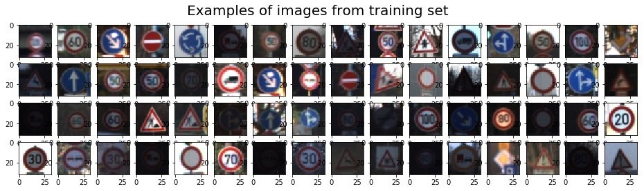
print("Number of classes =", n_classes)Number of training examples = 34799 Number of validation examples = 4410 Number of testing examples = 12630 Image data shape = (32, 32, 3) Number of classes = 43
Loading data
TRAFFIC SIGN CLASSIFICATION
import numpy as np
import matplotlib.pyplot as plt
import random
# Visualizations will be shown in the notebook.
get_ipython().magic('matplotlib inline')
def draw_images_examples(image_array, grid_x, grid_y, title):
fig = plt.figure(figsize=(grid_x,grid_y))
fig.suptitle(title, fontsize=20)
for i in range(1,grid_y*grid_x+1):
index = random.randint(0, len(image_array))
image = image_array[index].squeeze()
plt.subplot(grid_y,grid_x,i)
plt.imshow(image)
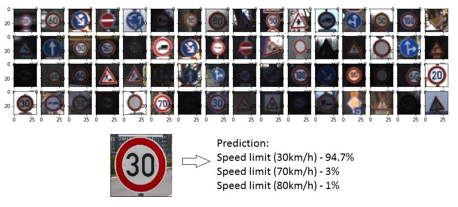
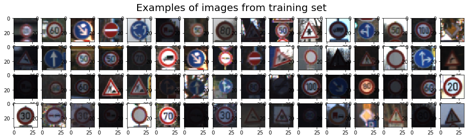
draw_images_examples(X_train, 16, 4, 'Examples of images from training set')
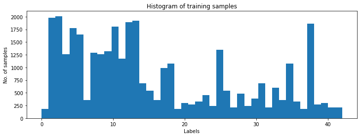
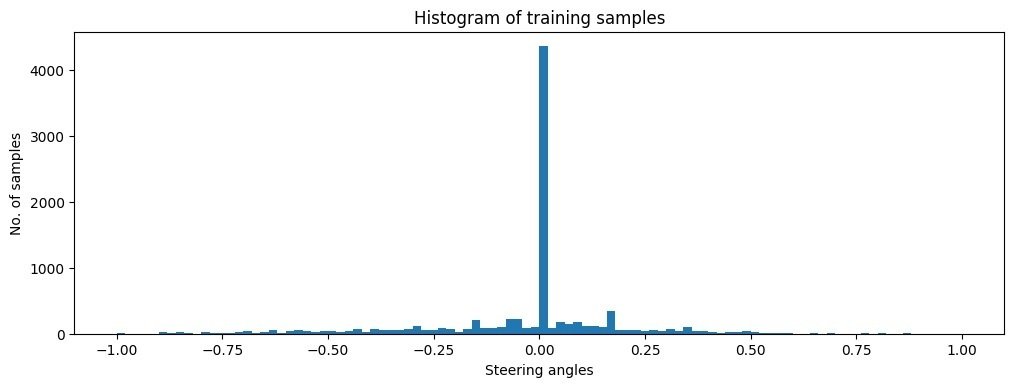
fig = plt.figure(figsize=(12,4))
n, bins, patches = plt.hist(y_train, n_classes)
plt.xlabel('Labels')
plt.ylabel('No. of samples')
plt.title('Histogram of training samples')
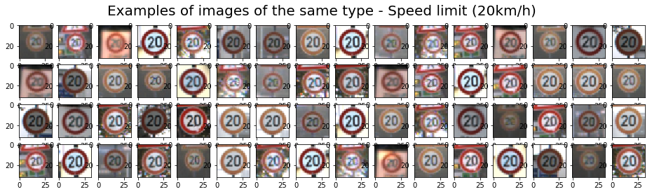
X_train_one_label = X_train[np.where(y_train==0)]
draw_images_examples(X_train_one_label, 16, 4, 'Examples of images of the same type - Speed limit (20km/h)')Data exploration
IMPLEMENTATION
TRAFFIC SIGN CLASSIFICATION
IMPLEMENTATION
TRAFFIC SIGN CLASSIFICATION
    def augment_brightness_camera_images(image):
        image1 = cv2.cvtColor(image,cv2.COLOR_RGB2HSV)
        random_bright = .25+np.random.uniform()
        image1[:,:,2] = image1[:,:,2]*random_bright
        image1 = cv2.cvtColor(image1,cv2.COLOR_HSV2RGB)
        return image1

    def transform_image(img):
        ang_range = 25
        ang_rot = np.random.uniform(ang_range)-ang_range/2
        rows,cols,ch = img.shape
        Rot_M = cv2.getRotationMatrix2D((cols/2,rows/2),ang_rot,1)

        img = cv2.warpAffine(img,Rot_M,(cols,rows))
        img = augment_brightness_camera_images(img)

        return img
Data augmentation
IMPLEMENTATION
Train set increased from 34799 to 139148
TRAFFIC SIGN CLASSIFICATION
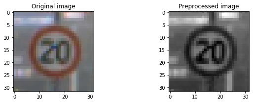
def grayscale(img):
return cv2.cvtColor(img, cv2.COLOR_RGB2GRAY)[:,:,None]
def normalize(value):
return value / 255 * 2 - 1
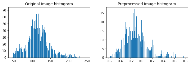
def preprocess_image(image):
img = grayscale(image)
img = normalize(img)
return imgData preprocessing
IMPLEMENTATION
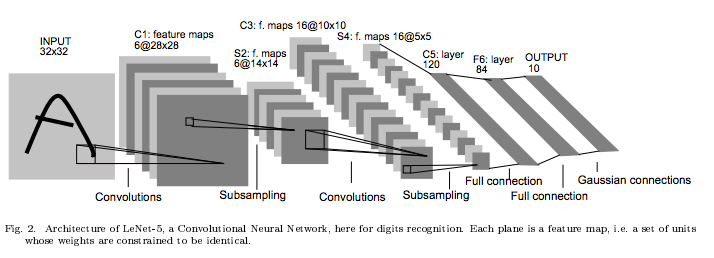
TRAFFIC SIGN CLASSIFICATION
Convolutional Neural Network
IMPLEMENTATION
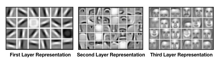
from: https://killianlevacher.github.io/blog/posts/post-2016-03-01/img/layeredRepresentation.jpg
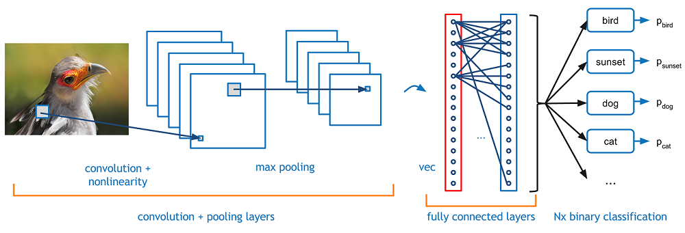
https://adeshpande3.github.io/adeshpande3.github.io/A-Beginner%27s-Guide-To-Understanding-Convolutional-Neural-Networks/
TRAFFIC SIGN CLASSIFICATION
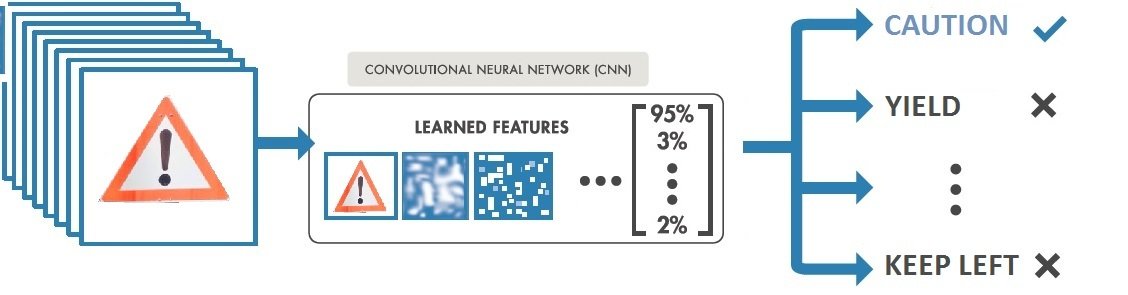
Convolutional Neural Network
IMPLEMENTATION
from: https://killianlevacher.github.io/blog/posts/post-2016-03-01/img/layeredRepresentation.jpg
TRAFFIC SIGN CLASSIFICATION
Convolutional Neural Network
IMPLEMENTATION
    import tensorflow as tf
    from tensorflow.contrib.layers import flatten


    # Arguments used for tf.truncated_normal, randomly defines variables for the weights and biases for each layer
    mu = 0
    sigma = 0.1

    # Layer 1: Convolutional. Input = 32x32x1. Output = 28x28x6.
    conv1_W = tf.Variable(tf.truncated_normal(shape=(5, 5, 3, 6), mean = mu, stddev = sigma))
    conv1_b = tf.Variable(tf.zeros(6))
    conv1   = tf.nn.conv2d(x, conv1_W, strides=[1, 1, 1, 1], padding='VALID') + conv1_b

    # Activation.
    conv1 = tf.nn.relu(conv1)

    # Pooling. Input = 28x28x6. Output = 14x14x6.
    conv1 = tf.nn.avg_pool(conv1, ksize=[1, 2, 2, 1], strides=[1, 2, 2, 1], padding='VALID')

    # Layer 2: Convolutional. Output = 10x10x16.
    conv2_W = tf.Variable(tf.truncated_normal(shape=(5, 5, 6, 16), mean = mu, stddev = sigma))
    conv2_b = tf.Variable(tf.zeros(16))
    conv2   = tf.nn.conv2d(conv1, conv2_W, strides=[1, 1, 1, 1], padding='VALID') + conv2_b

    # Activation.
    conv2 = tf.nn.relu(conv2)

    # Pooling. Input = 10x10x16. Output = 5x5x16.
    conv2 = tf.nn.avg_pool(conv2, ksize=[1, 2, 2, 1], strides=[1, 2, 2, 1], padding='VALID')
TRAFFIC SIGN CLASSIFICATION
Convolutional Neural Network
IMPLEMENTATION
    # Flatten. Input = 5x5x16. Output = 400.
    fc0   = flatten(conv2)

    # Layer 3: Fully Connected. Input = 400. Output = 120.
    fc1_W = tf.Variable(tf.truncated_normal(shape=(400, 120), mean = mu, stddev = sigma))
    fc1_b = tf.Variable(tf.zeros(120))
    fc1   = tf.matmul(fc0, fc1_W) + fc1_b

    # Activation.
    fc1    = tf.nn.relu(fc1)

    # Layer 4: Fully Connected. Input = 120. Output = 84.
    fc2_W  = tf.Variable(tf.truncated_normal(shape=(120, 84), mean = mu, stddev = sigma))
    fc2_b  = tf.Variable(tf.zeros(84))
    fc2    = tf.matmul(fc1, fc2_W) + fc2_b

    # Activation.
    fc2    = tf.nn.relu(fc2)

    # Layer 5: Fully Connected. Input = 84. Output = 43.
    fc3_W  = tf.Variable(tf.truncated_normal(shape=(84, n_classes), mean = mu, stddev = sigma))
    fc3_b  = tf.Variable(tf.zeros(n_classes))
    logits = tf.matmul(fc2, fc3_W) + fc3_b

    return logits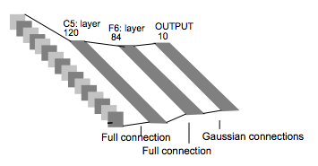
TRAFFIC SIGN CLASSIFICATION
CNN Training
IMPLEMENTATION
    from sklearn.utils import shuffle

    EPOCHS = 100
    BATCH_SIZE = 128

    with tf.Session() as sess:
        sess.run(tf.global_variables_initializer())
        num_examples = len(X_train_processed)

        print("Training...")
        print()
        for i in range(EPOCHS):
            X_train_processed, y_train = shuffle(X_train_processed, y_train)
            for offset in range(0, num_examples, BATCH_SIZE):
                end = offset + BATCH_SIZE
                batch_x, batch_y = X_train_processed[offset:end], y_train[offset:end]
                train_op, cost = sess.run([training_operation, loss_operation], feed_dict={x: batch_x, y: batch_y})

            validation_accuracy = evaluate(X_valid_processed, y_valid)
            print("EPOCH; {}; Valid.Acc.; {:.3f}; Loss; {:.5f}".format(i+1, validation_accuracy, cost))
            cost_arr.append(cost)


        saver.save(sess, './lenet')
        print("Model saved")
Feeding the model with batches of samples
TRAFFIC SIGN CLASSIFICATION
RESULTS
- Initial LeNet model - 91 %
- Input images normalization - ~91 %
- Training set augmantation - 93 %
- Learn rate optimization - 95 %
- Finding optimum image transformations during training set augmentation - 96 %
- Trying different pool methods, dropout, choosing L2 loss, tuning learn rate again - 96.8
Methodology
Final results
- Training set accuracy of 99.5 %
- Validation set accuracy of 96.8 %
- Test set accuracy of 94.6 %
TRAFFIC SIGN CLASSIFICATION
RESULTS

Speed limit (30km/h)
Bumpy road
General caution
Keep right
No entry
Slippery road
Predictions:
Probability:
94%
99%
100%
100%
100%
99%
3% for - Speed limit (30km/h)
TRAFFIC SIGN CLASSIFICATION
RESULTS
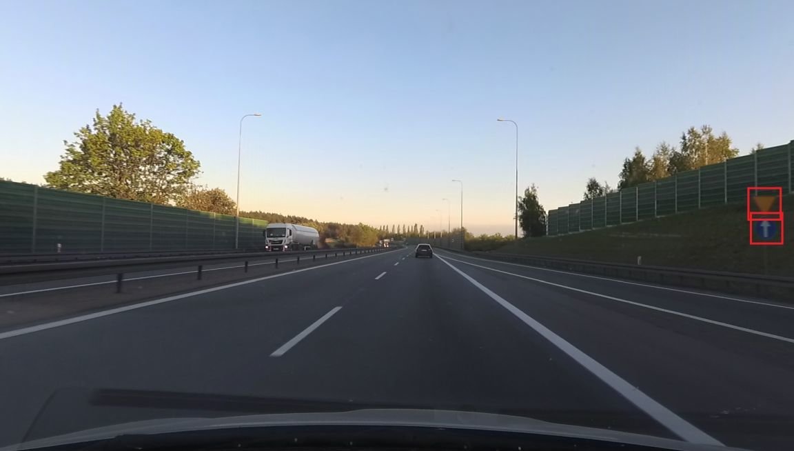
Test samples from Polish roads
TRAFFIC SIGN CLASSIFICATION
RESULTS
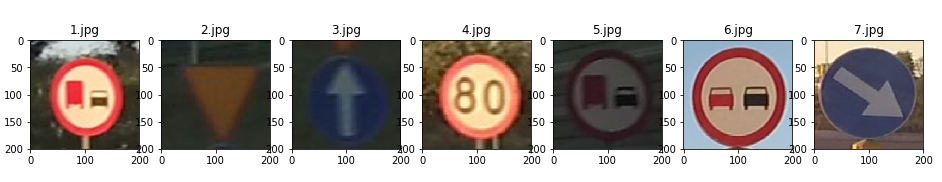
No passing for vehicles
over 3.5 metric tons
Yield
Ahead only
Speed limit (50km/h)
No passing for vehicles
over 3.5 metric tons
Ahead only
Keep right
100%
100%
99%
100%
92%
89%
45%
6.4% for - Speed limit (80km/h)
8.3% for - End of no passing
by vehicles over 3.5 metric tons
39% for - Turn right ahead
12% for - No vehicles
1.3% for - End of all speed and passing limits
Test samples from Polish roads
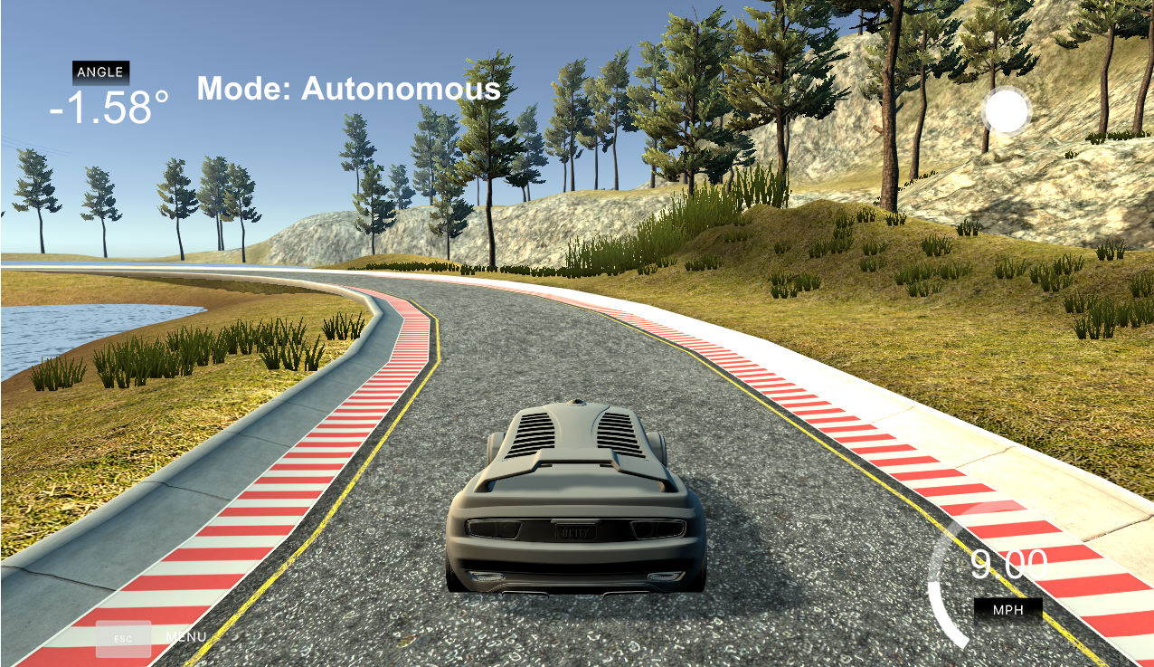
BEHAVIORAL
CLONING

BEHAVIORAL
CLONING
Collect data of driving behavior
Build CNN which predicts
steering angles
Train and validate the model
Test the model
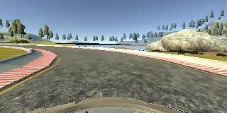
DATA COLLECTION
BEHAVIORAL CLONING
DATA COLLECTION
BEHAVIORAL CLONING
DATA COLLECTION
BEHAVIORAL CLONING
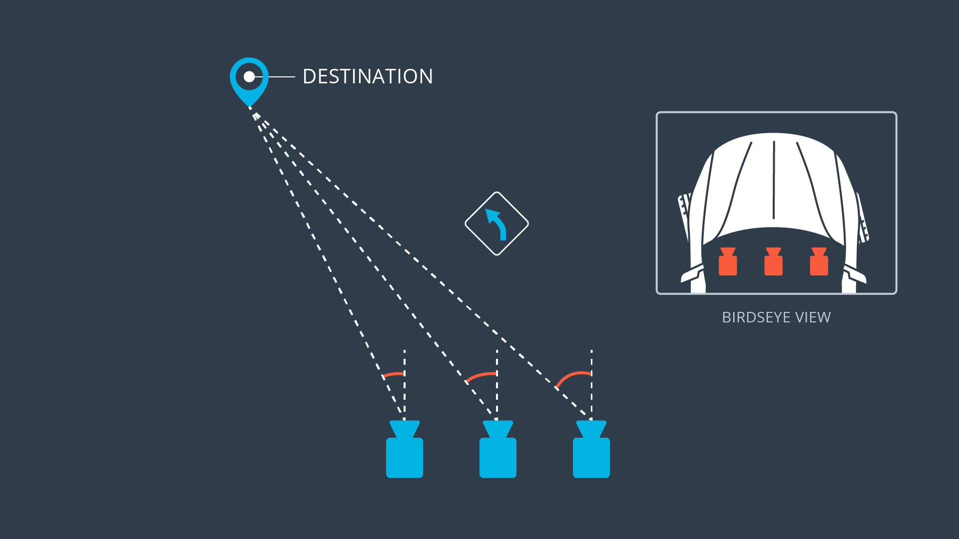
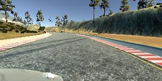
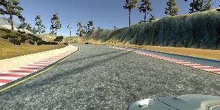
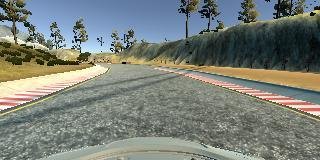
Left camera
Center camera
Right camera
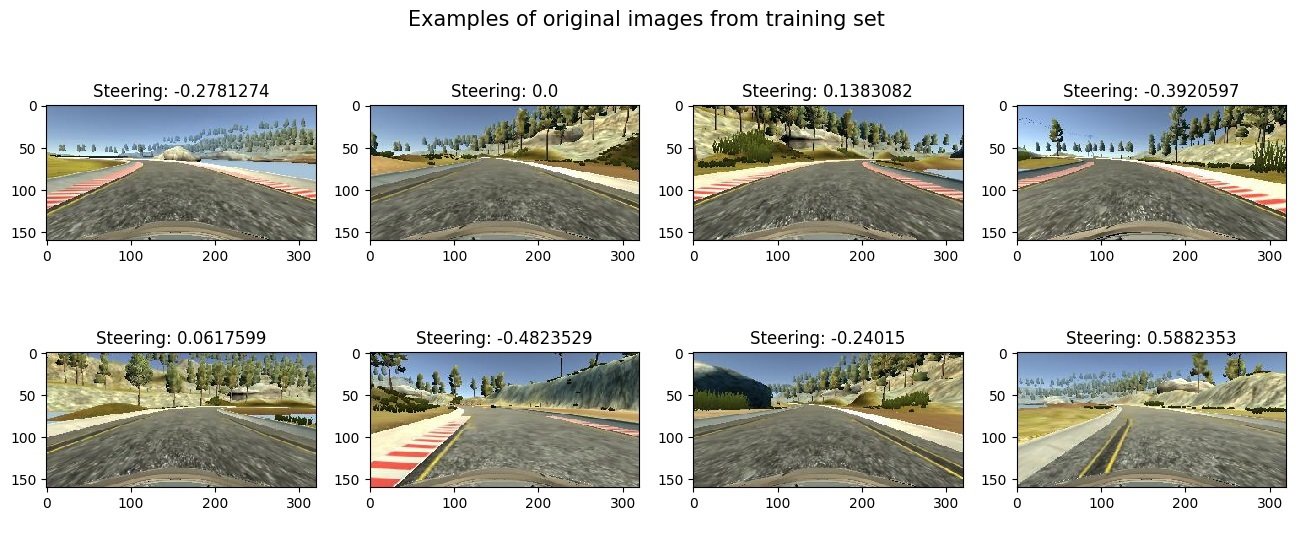
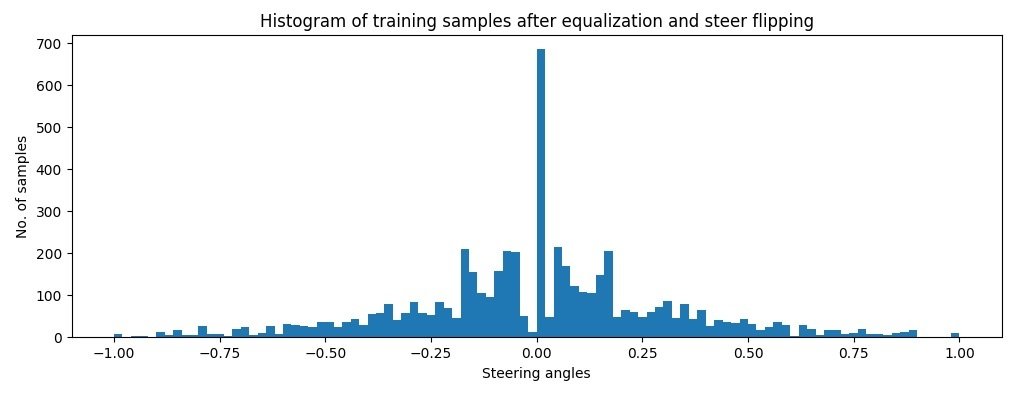
DATA AUGMENTATION
BEHAVIORAL CLONING
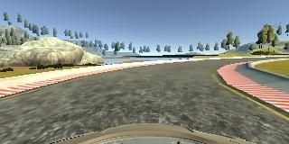
Original image
Flipped image
DATA AUGMENTATION
BEHAVIORAL CLONING
CONVOLUTIONAL NEURAL NETWORK
BEHAVIORAL CLONING
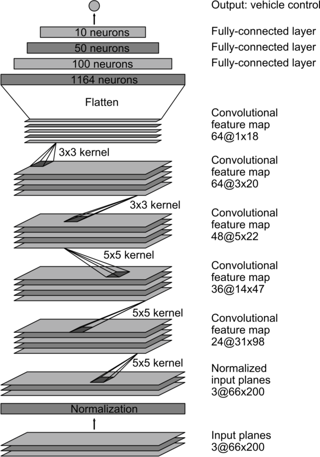
from: https://devblogs.nvidia.com/parallelforall/deep-learning-self-driving-cars/
27 million connections
250 thousand parameters
def build_nvidia_model(dropout=.4):
    model = Sequential()
    input_shape_before_crop=(IMAGE_ROWS_BEFORE_CROP,IMAGE_COLS, CHANNELS)
    input_shape_after_crop=(IMAGE_ROWS, IMAGE_COLS, CHANNELS)
    # trim image to only see section with the road
    model.add(Cropping2D(cropping=((IMAGE_CROP_TOP,IMAGE_CROP_BOTTOM), (0,0)),\
        input_shape=input_shape_before_crop))
    # pixels normalization using Lambda method
    model.add(Lambda(lambda x: x/127.5-1, input_shape=input_shape_after_crop))

    model.add(Conv2D(24, (5, 5), activation='elu', strides=(2, 2)))
    model.add(Dropout(dropout))
    model.add(Conv2D(36, (5, 5), activation='elu', strides=(2, 2)))
    model.add(Dropout(dropout))
    model.add(Conv2D(48, (5, 5), activation='elu', strides=(2, 2)))
    model.add(Dropout(dropout))
    model.add(Conv2D(64, (3, 3), activation='elu'))
    model.add(Dropout(dropout))
    model.add(Conv2D(64, (3, 3), activation='elu'))
    model.add(Dropout(dropout))
    model.add(Flatten())
    model.add(Dense(100, activation='elu'))
    model.add(Dense(50, activation='elu'))
    model.add(Dense(10, activation='elu'))
    model.add(Dense(1))

    optimizer = Adam(lr=0.001)
    model.compile(optimizer=optimizer,
                  loss='mse')
    return model
from keras.models import Sequential
from keras.layers import Dense, Dropout, Flatten, Lambda
from keras.layers import Conv2D, Cropping2D
from keras.optimizers import AdamArchitecture from Nvidia
IMPLEMENTATION
BEHAVIORAL CLONING
    BATCH_SIZE = 128
    NO_EPOCHS = 3

    train_generator = generator(train_samples, BATCH_SIZE, ANGLE_CORRECTION)
    validation_generator = generator(validation_samples, BATCH_SIZE, ANGLE_CORRECTION)

    model = build_nvidia_model()

    model.fit_generator(train_generator, steps_per_epoch=len(train_samples)/BATCH_SIZE, \
                        epochs=NO_EPOCHS, validation_data=validation_generator, \
                        validation_steps=len(validation_samples)/BATCH_SIZE)

    model.save('model.h5')
Model building
CONVOLUTIONAL NEURAL NETWORK
BEHAVIORAL CLONING
    def generator(samples, batch_size, angle_correction):
        num_samples = len(samples)
        angle_corrections = [0, angle_correction, -angle_correction]

        while 1: # Loop forever so the generator never terminates
            shuffle(samples)
            for offset in range(0, num_samples, batch_size):
                batch_samples = samples[offset:offset+batch_size]

                images = []
                angles = []
                for batch_sample in batch_samples:
                    camera_index = get_camera_index()
                    image = get_image_from_sample_line(batch_sample, camera_index, resizing=True)
                    steering = float(batch_sample[3]) + angle_corrections[camera_index]

                    image, steering = flip_image_and_steering(image, steering)

                    images.append(image)
                    angles.append(steering)

                X_train = np.array(images)
                y_train = np.array(angles)
                yield sklearn.utils.shuffle(X_train, y_train)
Generators
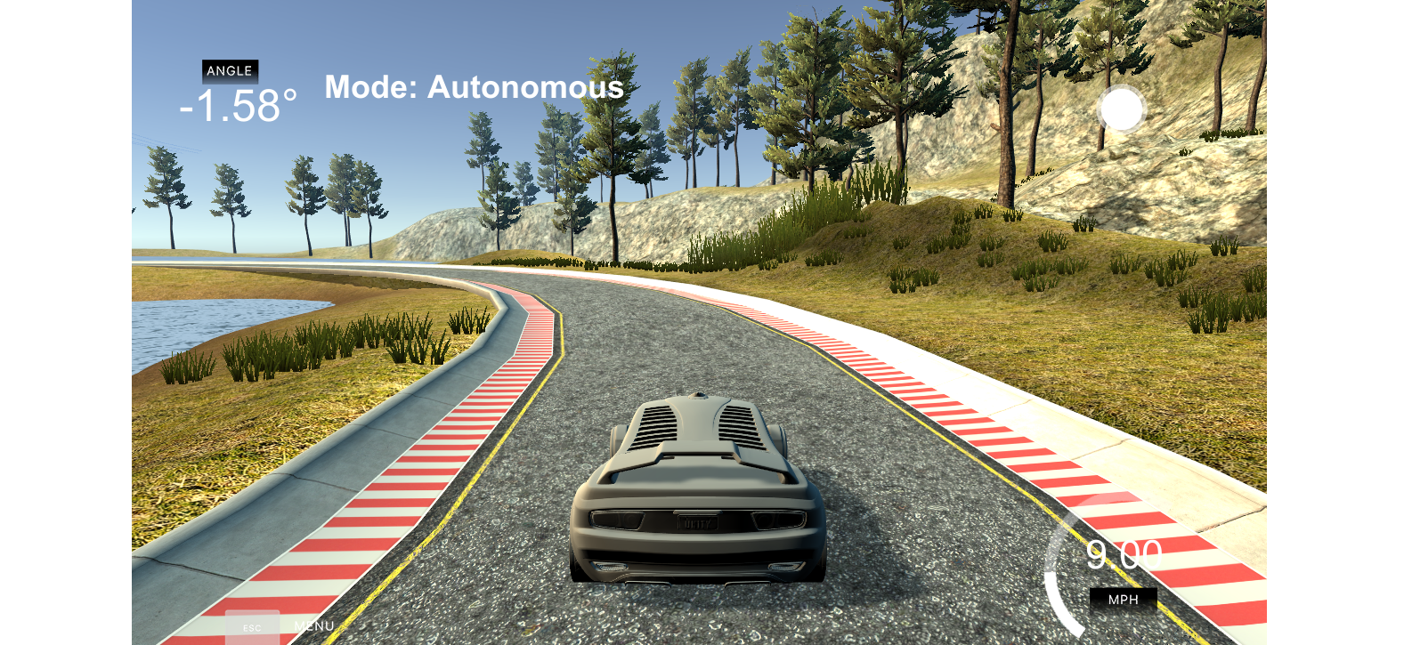
RESULTS
BEHAVIORAL CLONING
SUMMARY

Thank
You!
www.tomaszkacmajor.pl
tomasz.kacmajor@gmail.com
Trójmiasto
All code for the presented projects available on https://github.com/tomaszkacmajor
Self-Driving Cars with Python
By Tomasz Kacmajor