Online Kernel Matrix Factorization


Ing. Andrés Esteban Páez Torres
Director:
Fabio Augusto González Osorio PhD.
Motivation-Matrix Factorization
MF is a powerful analysis tool. Has applications like clustering, latent topic analysis, dictionary learning, among others.
Motivation-Kernel methods
Kernel methods allow extracting non-linear patterns from data, however have a high space and time cost compared to linear methods
Motivation-Large scale
The amount of aviable information is growing fast and there are many opportunities analysing this information.

Matrix Factorization
Matrix factorization is a family of linear-algebra methods that take a matrix and compute two or more matrices, when multiplied are equal to the input matrix
X
=
W
H
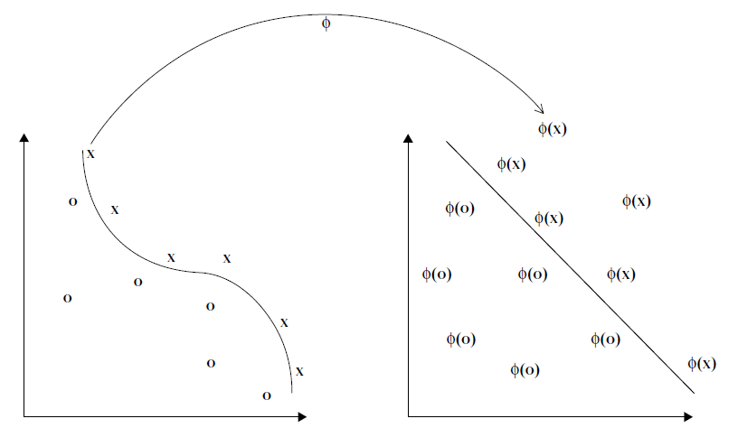
Kernel Method
\Phi:\mathcal{X}\longmapsto\mathcal{F}
\Phi:x\longmapsto\Phi(x)
Kernels are functions that map points from a input space X to a feature space F where the non-linear patterns become linear
Kernel Method (cont.)
Kernel Trick
- Many methods can use inner-products instead of actual points.
- We can find a function that calculates the inner-product for a pair of points in feature space
k(x,y)=\langle\Phi(x),\Phi(y)\rangle
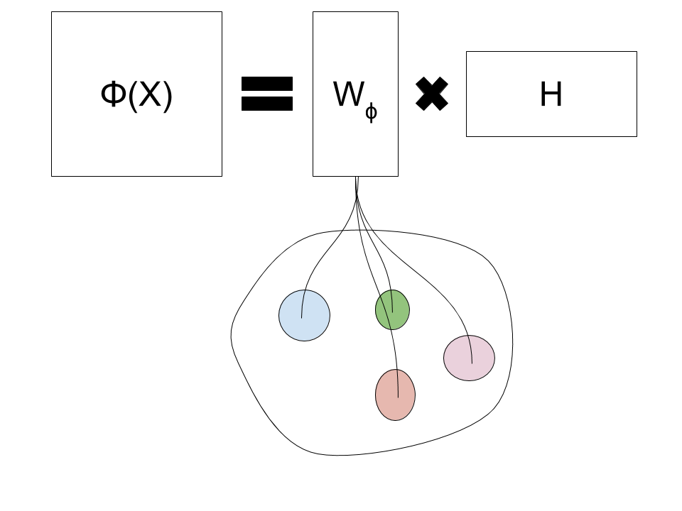
Kernel Matrix Factorization
Kernel Matrix factorization is a similar method, however, instead of factorizing the input-space matrix, it factorizes a feature-space matrix.
\Phi(X)
=
W_\phi
H
Problem-Explicit mapping
Usually isn't possible to calculate the explicit mapping into feature space. There are feature spaces with infinte dimensions or are just unkown.
X\longmapsto \Phi(X)
/
Problem-Large Scale Kernel Trick
Using the kernel trick is easier, however, computing a pairwise kernel function, leads to a Gram matrix of size n×n and a computing time O(n²)
n\times n
\Phi(X)^T\Phi(X)
Main Objective
To design, implement and evaluate a new KMF method that is able to compute an kernel-induced feature space factorization to a large-scale volume of data
Specific Objectives
- To adapt a matrix factorization algorithm to work in a feature space implicitly defined by a kernel function.
- To design and implement an algorithm which calculates a kernel matrix factorization using a budget restriction.
- To extend the in-a-budget kernel matrix factorization algorithm to do online learning.
- To evaluate the proposed algorithms in a particular task that involves kernel matrix factorization.
Contributions
- Design of a new KMF algorithm, called online kernel matrix factorization (OKMF).
- Efficient implementation of OKMF using CPU and GPU.
- Online Kernel Matrix Factorization. Conference article presented at XX Congreso Iberoamericano de Reconocimiento de Patrones 2015.
- Accelerating kernel matrix factorization through Theano GPGPU symbolic computing. Article to be published.
Factorization
\Phi(X)=\Phi(B)WH
\Phi(X)\in \mathbb{R}^{l\times n}
\Phi(B)\in \mathbb{R}^{l\times p}
W\in \mathbb{R}^{p\times r}
H\in \mathbb{R}^{r\times n}
p\ll n
About the Budget
- The budget matrix is a set of representative points ordered as columns.
- The budget selection is made through random picking o p X matrix or by computing k-means with k=p.
\Phi(B)\in \mathbb{R}^{l\times \red{p}}
Loss Function
\displaystyle
J(W,H)=\frac{1}{2}\|\Phi(X)-\Phi(B)WH\|^2_F+\frac{\lambda}{2}\|W\|^2_F+\frac{\alpha}{2}\|H\|^2_F
First Tackle-Explicit Mapping
\frac{1}{2}Tr(\Phi(X)^T\Phi(X))
-\frac{1}{2}Tr(2\Phi(X)^T\Phi(B)WH)
+\frac{1}{2}Tr(H^TW^T\Phi(B)^T\Phi(B)WH)
\text{All terms }\Phi(A)^T\Phi(C)\text{ can be replaced with a function }
K(A,C) = \{k(A_{i,:},C_{:,j})\}_{i,j}\text{, i.e. a matrix of the pairwise}
\text{inner-products of A and C in feature space.}
+...
Second Tackle-Large Scale Kernel Trick
\frac{1}{2}Tr(\Phi(X)^T\Phi(X))
-\frac{1}{2}Tr(2\Phi(X)^T\Phi(B)WH)
+\frac{1}{2}Tr(H^TW^T\Phi(B)^T\Phi(B)WH)
\text{Given all terms that contain matrices }W \text{ and } H\text{ have kernel}
+...
\text{matrices in terms of } \Phi(B)\text{ we can lower the memory required from}
O(n^2)\text{ to }O(np)
SGD Optimization Problem
\displaystyle
\frac{1}{2}\sum^n_{i=0}\|\Phi(x_i)-\Phi(B)Wh_i\|^2+\frac{\lambda}{2}\|W\|^2_F+\frac{\alpha}{2}\sum^n_{i=0}\|h_i\|^2
We selected SGD as the optimization technique, given the original loss function can be expressed as the following sum.
SGD Update Rules
\displaystyle
h_t = (W^T_{t-1}K(B,B)W_{t-1}-\alpha I)^{-1}W^T_{t-1}K(B,x_t)
\displaystyle
W_t = W_{t-1} - \gamma(K(B,x_t)h^T_t-K(B,B)W_{t-1}h_th_t^T+\lambda W_{t-1})
Taking the partial derivative respect h and equalling to 0, we have:
Taking the partial derivative respect W and substracting it to W, we have:
The Final Tackle-Online+Budget
\text{Applying SGD, we can lower the amount of required memory}
\text{from }O(np) \text{ to }O(p^2)\text{ which is a lot lower if }p\ll n\text{.}
\text{Given SDG approximates the true gradient of the loss function}
\text{using a sample at the time, rather than computing it for every}
\text{sample in the dataset, OKMF is faster than a batch gradient}
\text{descent algorithm.}
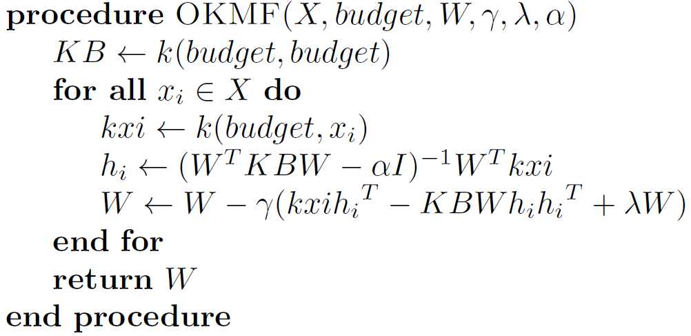
OKMF Algorithm
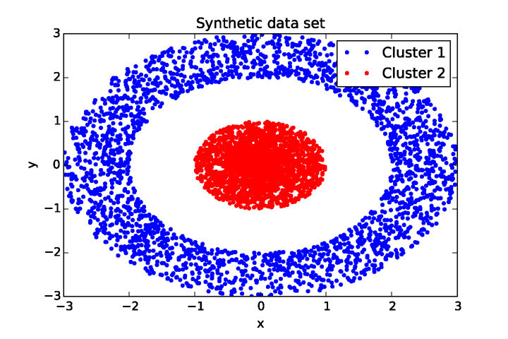
Experimental Evaluation
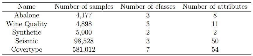
- A clustering task was selected to evaluate OKMF
- 5 data sets were selected, raging from 4177 to 58012 instances.
Performance Measure
The selected performance measure is the clustering accuracy, this measures the ratio between the number of correctly clustered instances and the total number of instances.
- Calculate the confusion matrix
- Substract the confision matrix from a big value
- Apply the Hungarian algorithm to the resulting matrix
- Substract the big value to the reordered matrix, change the sign.
- Calculate the trace of the resulting matrix and divide in the total number of instances.
Compared Algorithms
- Kernel k-means
- Kernel convex non-negative factorization
- Online k-means (no kernel)
- Online kernel matrix factorization
Used Kernel Functions
Linear kernel
k(x,y)=x^Ty
Gaussian kernel
k(x,y)=\exp(-\frac{\|x-y\|^2}{2\sigma^2})
Parameter Tuning
- The learning rate, regularization and Gaussian parameters were tuned for OKMF in order to minimize the average loss of 10 runs.
- The Gaussian kernel parameter was tuned fro CNMF and Kernel k-means to maximize the average accuracy of 10 runs.
- The budget size of OKMF was fix to 500 instances
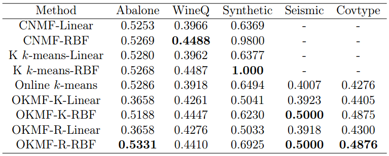
Results
- The experiments consists of 30 runs, the average clustering accuracy and average clustering time are reported.
Average Clustering Accuracy of 30 runs
Average Clustering Time of 30 runs (seconds)

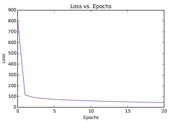
Loss vs. Epochs
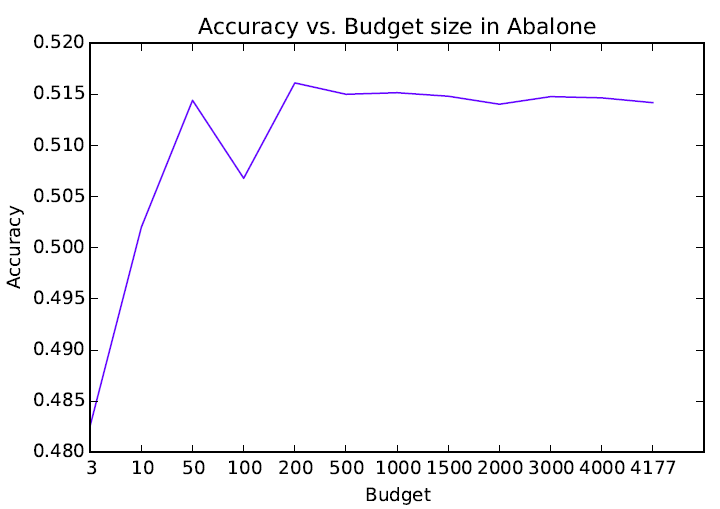
Accuracy vs. Budget Size
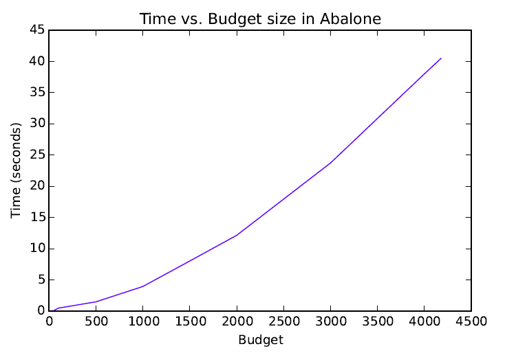
Time vs. Budget Size
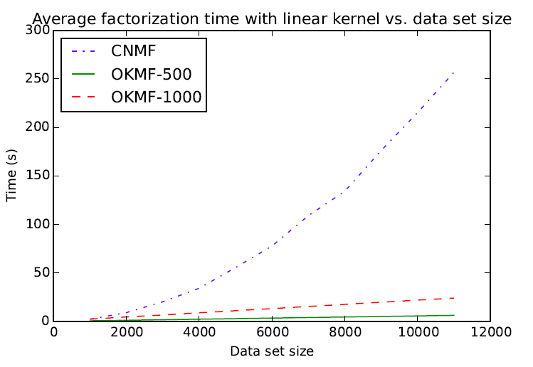
Avg. factorization time vs. dataset size (linear)
Conclusions
- OKMF is a memory efficient algorithm, it requires to store a matrix, which is better than a matrix if
- Also, SGD implies a memory saving, given OKMF stores a vector of size instead of a matrix of size
n\times n
p\times p
p\ll n
p
p\times n
Conclusions (cont.)
- OKMF has a competitive performance compared with other KMF and clustering algorithms in the clustering task.
- Exprimental results show OKMF can scale linearly with respect the number of instances.
- Finally, the budget selection schemes tested were equivalent, so isn't necessary the extra computation of k-means cluster centers.
Final Thesis Defense Presentation
By Andres Esteban Paez Torres
Final Thesis Defense Presentation
My thesis presentation