egp@vt.edu
Eric Paterson is Professor and Department Head of Aerospace and Ocean Engineering. For Fall 2013, he is teaching AOE 5984, Intro to Parallel Computing Applications with faculty from Virginia Tech's Advanced Research Computing.
[03:03:53][egp@egpMBP:parallelProcessing]542$ pwd
/Users/egp/OpenFOAM/OpenFOAM-2.2.x/applications/utilities/parallelProcessing
[03:04:09][egp@egpMBP:parallelProcessing]543$ ls -l
total 0
drwxr-xr-x  3 egp  staff  918 May 17 09:51 decomposePar
drwxr-xr-x  3 egp  staff  204 May 17 09:51 reconstructPar
drwxr-xr-x  3 egp  staff  170 May 17 09:52 reconstructParMesh
drwxr-xr-x 3 egp staff 272 May 17 09:52 redistributePar 
numberOfSubdomains 64; [03:41:22][egp@brlogin1:simpleFoam]13058$ cp -rf pitzDaily pitzDailyParallel[03:42:42][egp@brlogin1:pitzDailyParallel]13066$ cp $FOAM_UTILITIES/parallelProcessing/decomposePar/decomposeParDict system/.
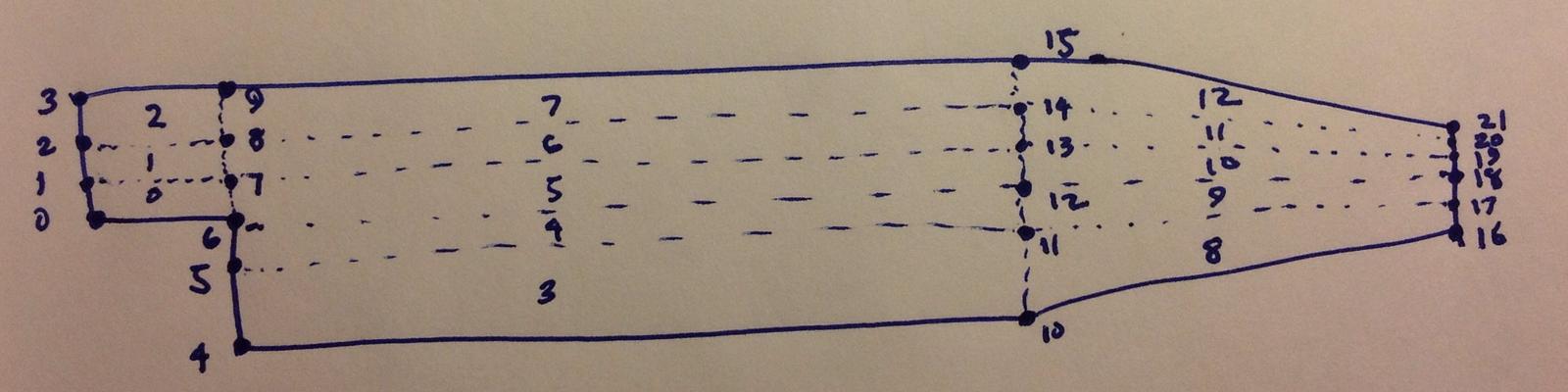
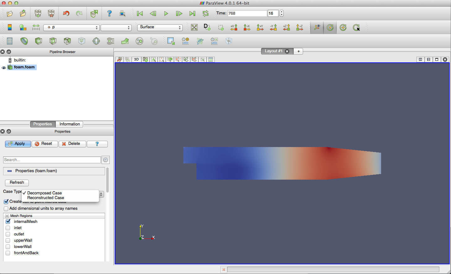
pitzDaily Backward Facing Step tutorial
[05:12:36][egp@brlogin1:pitzDailyParallel]13097$ decomposePar -cellDist
/*---------------------------------------------------------------------------*\
| =========                 |                                                 |
| \\      /  F ield         | OpenFOAM: The Open Source CFD Toolbox           |
|  \\    /   O peration     | Version:  2.2.0                                 |
|   \\  /    A nd           | Web:      www.OpenFOAM.org                      |
|    \\/     M anipulation  |                                                 |
\*---------------------------------------------------------------------------*/
Build  : 2.2.0
Exec   : decomposePar -cellDist
Date   : Nov 14 2013
Time   : 05:12:46
Host   : "brlogin1"
PID    : 61396
Case   : /home/egp/OpenFOAM/egp-2.2.0/run/tutorials/incompressible/simpleFoam/pitzDailyParallel
nProcs : 1
sigFpe : Floating point exception trapping - not supported on this platform
fileModificationChecking : Monitoring run-time modified files using timeStampMaster
allowSystemOperations : Disallowing user-supplied system call operations

// * * * * * * * * * * * * * * * * * * * * * * * * * * * * * * * * * * * * * //
Create time


Decomposing mesh region0

Removing 4 existing processor directories
Create mesh

Calculating distribution of cells
Selecting decompositionMethod scotch

Finished decomposition in 0.07 s

Calculating original mesh data

Distributing cells to processors

Distributing faces to processors

Distributing points to processors

Constructing processor meshes

Processor 0
    Number of cells = 3056
    Number of faces shared with processor 1 = 86
    Number of faces shared with processor 2 = 60
    Number of processor patches = 2
    Number of processor faces = 146
    Number of boundary faces = 6222

Processor 1
    Number of cells = 3056
    Number of faces shared with processor 0 = 86
    Number of processor patches = 1
    Number of processor faces = 86
    Number of boundary faces = 6274

Processor 2
    Number of cells = 3065
    Number of faces shared with processor 0 = 60
    Number of faces shared with processor 3 = 57
    Number of processor patches = 2
    Number of processor faces = 117
    Number of boundary faces = 6237

Processor 3
    Number of cells = 3048
    Number of faces shared with processor 2 = 57
    Number of processor patches = 1
    Number of processor faces = 57
    Number of boundary faces = 6277

Number of processor faces = 203
Max number of cells = 3065 (0.286299% above average 3056.25)
Max number of processor patches = 2 (33.3333% above average 1.5)
Max number of faces between processors = 146 (43.8424% above average 101.5)


Wrote decomposition to "/home/egp/OpenFOAM/egp-2.2.0/run/tutorials/incompressible/simpleFoam/pitzDailyParallel/constant/cellDecomposition" for use in manual decomposition.

Wrote decomposition as volScalarField to cellDist for use in postprocessing.
Time = 0

Processor 0: field transfer
Processor 1: field transfer
Processor 2: field transfer
Processor 3: field transfer

End. method scotch;scotchCoeffs
{
} 
method          simple;simpleCoeffs
{
 (2 2 1);
    delta         n
   0.001;
} 
blocks
(
    hex (0 6 7 1 22 28 29 23) (18 7 1) simpleGrading (0.5 1.8 1)
    hex (1 7 8 2 23 29 30 24) (18 10 1) simpleGrading (0.5 4 1)
    hex (2 8 9 3 24 30 31 25) (18 13 1) simpleGrading (0.5 0.25 1)
    hex (4 10 11 5 26 32 33 27) (180 18 1) simpleGrading (4 1 1)
    hex (5 11 12 6 27 33 34 28) (180 9 1) edgeGrading (4 4 4 4 0.5 1 1 0.5 1 1 1 1)
    hex (6 12 13 7 28 34 35 29) (180 7 1) edgeGrading (4 4 4 4 1.8 1 1 1.8 1 1 1 1)
    hex (7 13 14 8 29 35 36 30) (180 10 1) edgeGrading (4 4 4 4 4 1 1 4 1 1 1 1)
    hex (8 14 15 9 30 36 37 31) (180 13 1) simpleGrading (4 0.25 1)
    hex (10 16 17 11 32 38 39 33) (25 18 1) simpleGrading (2.5 1 1)
    hex (11 17 18 12 33 39 40 34) (25 9 1) simpleGrading (2.5 1 1)
    hex (12 18 19 13 34 40 41 35) (25 7 1) simpleGrading (2.5 1 1)
    hex (13 19 20 14 35 41 42 36) (25 10 1) simpleGrading (2.5 1 1)
    hex (14 20 21 15 36 42 43 37) (25 13 1) simpleGrading (2.5 0.25 1)
); 
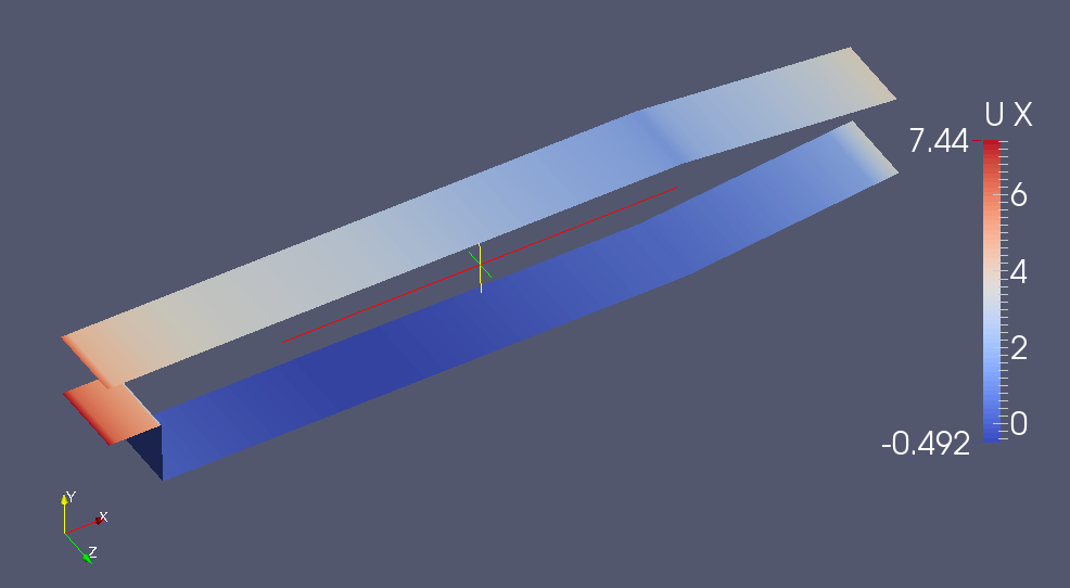
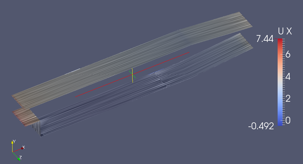
cp $FOAM_UTILITIES/postProcessing/sampling/sample/sampleDict system/.
mpirun -np 4 sample -latestTime -parallel
fields
(
    p
    U
    nut
    k
    epsilon
);
surfaces
(
nearWalls_interpolated
{
// Sample cell values off patch. Does not need to be the near-wall
// cell, can be arbitrarily far away.
type patchInternalField;
patches ( ".*Wall.*" );
interpolate true;
offsetMode normal;
distance 0.0001;
}
); sets
(
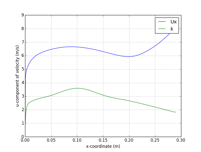
centerline
{
type midPointAndFace;
axis x;
start (0.0 0.0 0.0);
end (0.3 0.0 0.0);
}
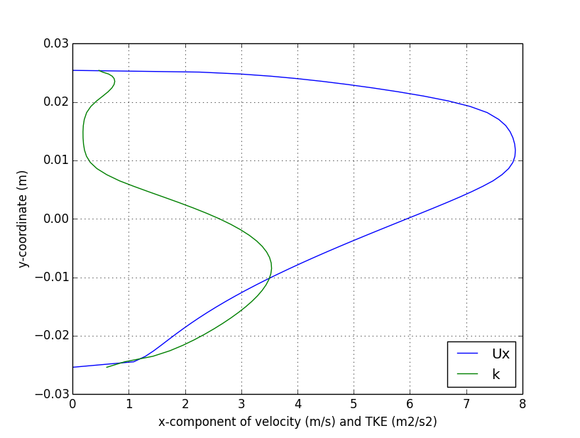
verticalProfile
{
type midPointAndFace;
axis y;
start (0.206 -0.03 0.0);
end (0.206 0.03 0.0);
}
); 
By egp@vt.edu
OpenFOAM for AOE 5984, Fall 2013. This lecture will cover parallel computing for OpenFOAM CFD simulations.


