


Hugo Hadfield
Cambridge University PhD student, Signal Processing and Communications Laboratory
Queens' College
Gonville and Caius College
Trinity College
Cambridge University Signal Processing and Communications Laboratory
Building algorithms to control robots is inherently geometric
Forward Kinematics is typically all about composing and chaining transformations (rotation and translation)
Inverse Kinematics requires finding intersections and reflections of geometric primitives (especially circles and spheres)
Conformal Geometric Algebra (CGA) combines many geometric primitives, intersections and transformations
Set up a bunch of orthogonal basis vectors, define the geometric product of a basis vector with itself, eg. for 3DGA
The multiplication of two orthogonal basis vectors anticommutes and we often use a shorthand to write it
If we now make two vectors and multiply them with the geometric product we can see what happens
The result of the geometric product has both terms that are scalars and terms that are the multiplication of two basis vectors
Let's define an operation, the grade selection operation
If there is nothing of the grade in there, then it gives 0
The result of the geometric product can be written with grade selection
Inner (dot) product
And this motivates us to define two new products...
Outer (wedge) product
Note: people define various different behaviours of the inner product with scalars
CGA creates two more basis vectors that square to +1 and -1 respectively:
\[ e_1^2 = 1, e_2^2 = 1, e_3^2 = 1, \bf{e_4^2 = 1, e_5^2 = -1} \]
We use the extra basis vectors to construct two null vectors *
Then use the null vectors to embed our 3D point in 5D
* Note, people use a range of different notations here in papers etc, it doesn't really matter what you use as long as you are consistent!
For more info see references [1,2]
This is not a random choice!
Dot product between points is proportional to the squared distance between them
The null vectors correspond to the origin and infinity!
Check:
Like in graphics programming where we work with 4D homogeneous coordinates, here we go to 5D for more power :)
Geometric primitives can be made by wedging points together (see [2,3])
Point
Point pair/line segment
Circle
Infinite line
Sphere
Infinite plane
Geometric primitives can be made from traditional parameterisations via their dual (see [2,3])
Point pair
line segment
Circle
Infinite line
Infinite plane
Sphere
The meet or vee operator does intersection: \( \vee \)
(see [2,3])
The meet (wrt \(I_5\)) is a linear operator, it is distributive and associative
Intersections can be chained easily
CGA transformations contain all the motors ie. rotation and translation, but they also contain scaling and inversion, (all angle preserving transformations)
Rotors can again be represented as the exponentiation of bivectors (Lie algebra -> Lie group mapping)
Can nicely chain and interpolate transformations
Almost everything is completely "covariant", ie. you can prove it at the origin and it will hold everywhere
Rotation rotor
Translation rotor
Scaling rotor
All rotors are applied the same way:
Reflections are done by sandwiching one object inside another
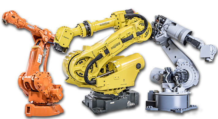
Serial robots have a series of joints, one after another
Known as a serial kinematic chain
Most common type of industrial robot
Building Cars
Colaborating with people
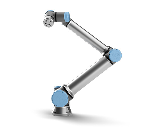
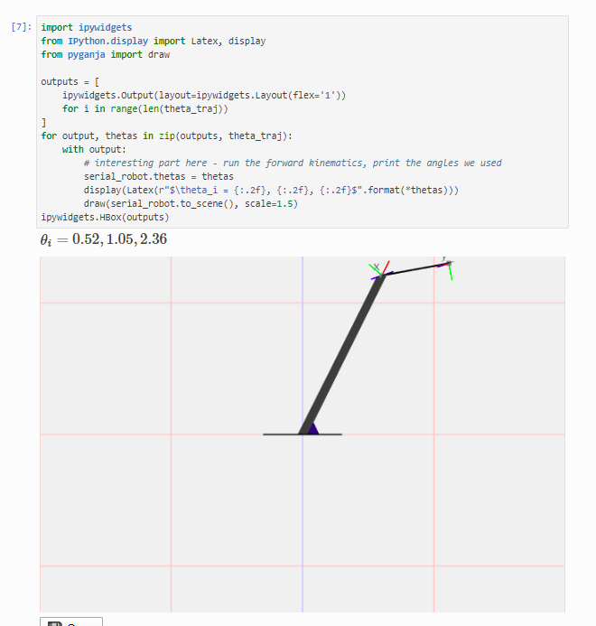
Consider a 2-link 3 degree of freedom serial robot arm
Where does the end point go as we change the motor angles?
Get the end point
Construct the base rotors
Get the elbow point
Construct the elbow rotor
What if we want the full orientation of the endpoint?
Can we construct a rotor from origin to endpoint?
Construct the base rotors
Construct the first link's translation rotor
Construct the elbow and link 2 translation rotor
The combined rotor is the product of all of them
(If \(P^2 < 0 \) then y is out of reach)
Construct a sphere at the base, \(n_0\)
Construct a sphere at the endpoint, y
Intersect the spheres to give a circle
Define a vertical plane through the endpoint and base
Intersect the circle and the plane to give a point pair
Choose one of the elbow position solutions
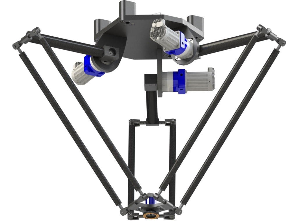
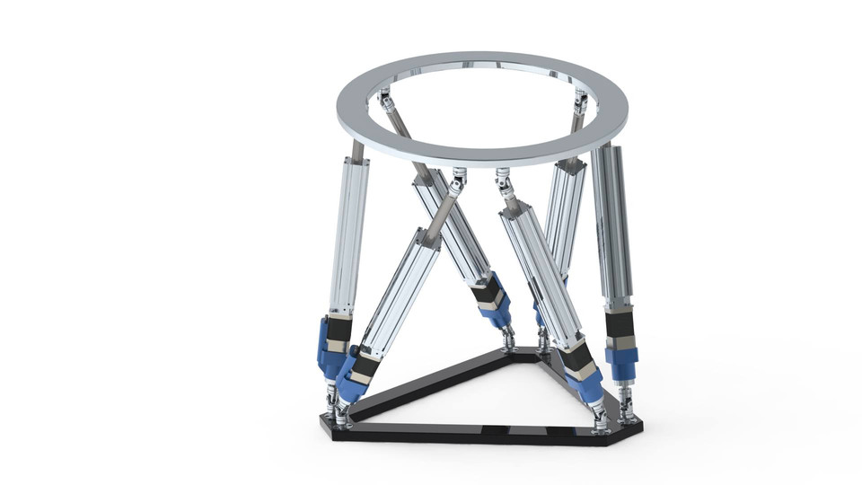
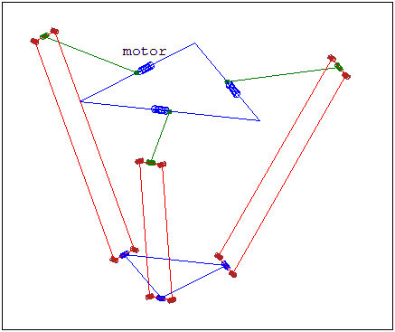
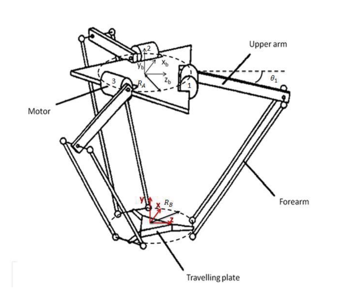
Parallel robots are composed of multiple kinematic chains
Inverse kinematics typically easy
Forward kinematics hard
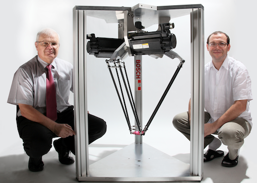
Delta Robot
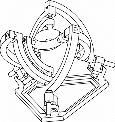
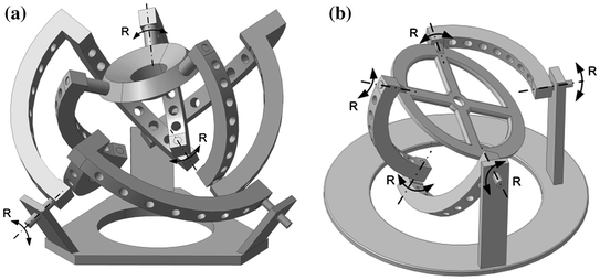
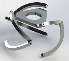
Agile Eye
Stewart Platform
The Agile Eye is a parallel robot originally designed for orienting cameras very quickly
(a) 3DoF Agile Eye
(b) 2DoF Agile Eye
2DoF version can change the orientation of the camera but cannot freely roll about the camera axis
Construct the drive rotors
Find the elbow points
Get the point pair on the camera plate
Get the normal to the plate
The axes of the motors all intersect at a single point, the centre of rotation
We define a rotation rotor R that fully defines the plate position
Each point on the plate defines an additional circle where the elbow could be
The fixed axis of each motor defines a fixed circle on which the elbow must lie
Get the pseudo-elbow point \(A_i\)
Construct a sphere about the pseudo-elbow
The intersection of the three spheres (one from each limb) correspond to the two possible possitions of the centre of the end plate
If \(T_i^2 < 0\) then the target point is unreachable
Construct three possible elbow position circles
Construct three possible elbow position spheres
Intersect each sphere with its corresponding circle and select one possible intersection solution per limb
Finally get the motor angles
Many GA operations are linear and chainable
Linear functions can be converted to matrices (if you so desire..)
Linearity is great for differentiation!
This turns out to be very useful for robotics
CALCULUS ON THE VERTICAL SLIDES BELOW
Move only one motor
- Now we need to know how the conformal endpoint of the point pair changes
- How does the 3D endpoint change with the conformal endpoint change? (derivative of 'down' function)
- We now have a closed form expression for the derivative of the endpoint wrt. theta and we didn't have to use maple once!
- We can use this for control and optimisation. Consider a cost function:
- We therefore have a closed form for
and so can do gradient descent
- Given the forward jacobian we can simply invert the 3x3 matrix at each point to get the inverse jacobian
OR
- We can differentiate our inverse kinematic equations..
Starting with \(\Sigma_i \)
Differentiate wrt. a scalar param \( \alpha \)
the sphere centred at the meeting of the 4 bar mechanism and the end platform
- Now we need to know how the elbow positions vary with \alpha
- Here \(A_i\) is the conformal elbow position
- Finally we need to know how the joints vary with elbow position
- We are done (Once again no Maple!)
- The inverse jacobian allows us to map velocity of the endpoint to velocity of joints
- In other words, to minimise cost at maximum rate drive the end point linearly at our target point (obviously)
- With the inverse jacobian we can do exactly that
So far we have dealt with geometry of robots, constraints and kinematics of the end effector
Now we would like to also deal more generally with statics and dynamics
Ideally our setup should be familiar/intuitive to robotics practitioners and researchers to make it easy to use.
Forces have a line of action, an orientation, and a magnitude
We can therefore naturally encode a force as an infinite line in CGA
force magnitude
force direction
3d point through which the line passes
Note we have used the dual construction of the line here, ie. F is a bivector
The conditions for static equilibrium of a body subject to external forces and moments:
No net linear force
No net moment
What does this mean for our CGA force line formulation?
What is the sum of two CGA force lines?
Another force line + something else.. (see [10])
Let's consider a simple case: two force lines in a plane
So when the force lines meet at a point the sum of lines is just another line, ie:
The resultant force line passes through p which is the point at which they intersect. It also points in the direction of, and has magnitude the same as, the vector sum \( \lambda_1\hat{m_1} + \lambda_2\hat{m_2}\):
So for parallel force lines:
But for anti-parallel force lines of equal magnitude:
Physically speaking, balanced anti-parallel forces create a pure moment
is the moment generated by the geometric arrangement of forces
OK so we know how to do forces and we have a representation of a moment, but how do we calculate the moment of a line about a point?
For a point P and dual force line \(F_1\) the moment bivector M is given by:
This again produces a moment bivector of the from: \( a\wedge n_{\infty} \) , where \(|a|\) is the magnitude of the moment and \(\hat{a}\) is the direction of the moment axis
Both dual force lines and our bivector moments are screws, and specifically because they carry forces/moments they are known as wrenches (see [12])
If h is 0 then we have a force line
Iif m is 0 magnitude we have a pure moment
The general form of a screw is:
We can add and subtract screws at will and we will still stay on the screw manifold
With both external moments \(M_j \) and forces \(F_i \) our static equilibrium equation is:
We could also think of all the force and moments as screws and so:
But what happens if they don't sum to 0?
And we can define a screw velocity \(\dot{B}\) such that:
We will define a screw momentum quantity, \(\Omega\),
such that the sum of external wrenches is its time derivative
where \(R\) is the rotor that transforms things from the body frame to the world frame (see [11,14])
Screw momentum and screw velocity are related by screw inertia (see [13])
We can quantify screw inertia by considering how much a wrench would effect the body if it was already moving in one of 6 specific ways, these movements are the Principal Screws of Inertia
What is the response if it is rotating about axis \(e_1\) or \(e_2\) or \(e_3\)?
What is the response if it is translating along axis \(e_1\) or \(e_2\) or \(e_3\)?
Principal screws of inertia
The screw inertia tensor \(M\) and its inverse \(M^-1\) map between screw velocity \(\dot{B_b}\) and screw momentum \(\Omega_b\) in the body frame (aligned with the principal axes)
Reciprocal principal screws of inertia
\(m\) is the body's mass
\(\gamma_i\) is the body's second moment of area about each axis
To integrate all our bits and bobs we will use a standard 4'th order Runge-Kutta method (RK4)
To use the RK4 method we need to define our state \(y\) and a function \(f\) that returns the derivative of that state at a given time t and an initial value of \(y\) to start the simulation off at \(t_0\)
Our goal will be to simulate a couple of interesting dynamics phenomena as a test of correctness
The state we track is the rotor \(R\) that transforms from the body frame to the world frame and the screw momentum \(\Omega\) in the world frame
The body is under the influence of a time varying wrench \(W_b\) expressed in the body frame
CGA combines primitives, intersections, transformations (+Lie groups, algebras) and easy derivatives (wrt scalars)
(C)GA is not some alien language, it is the tools and techniques you already know and love packaged with a common interface
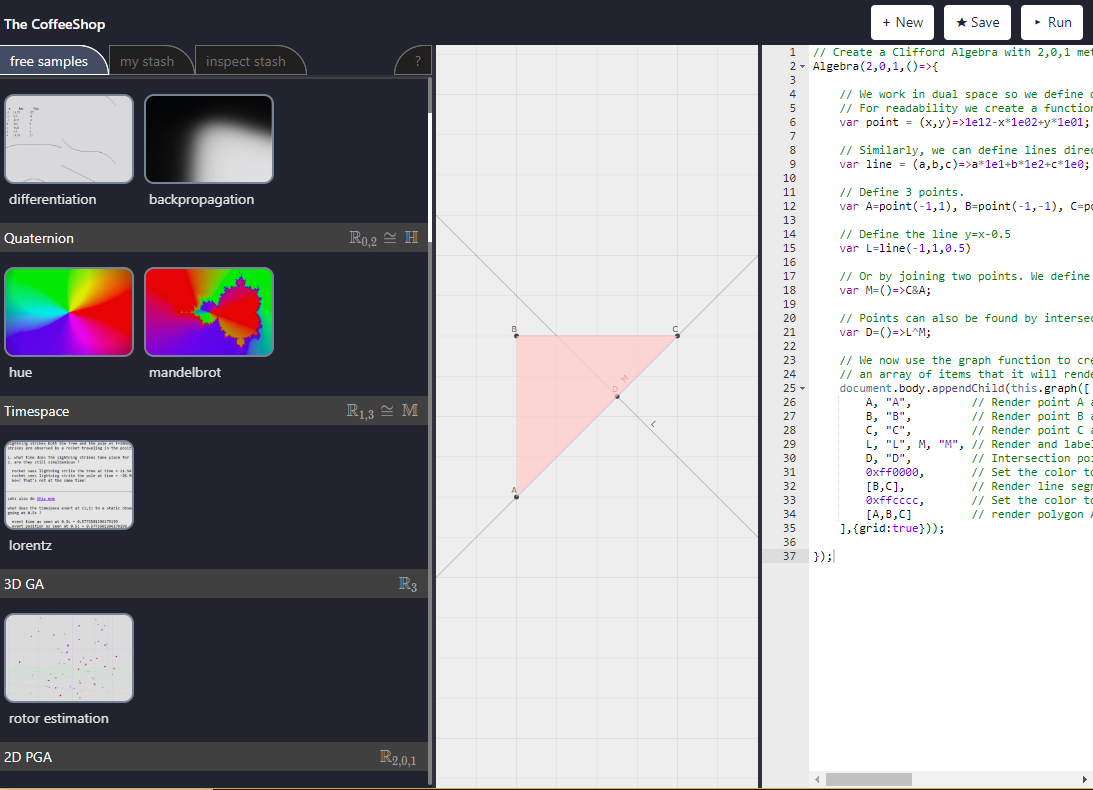
CGA is easy to work with and computationally feasable for real time applications (all the demos here are running in the browser!)
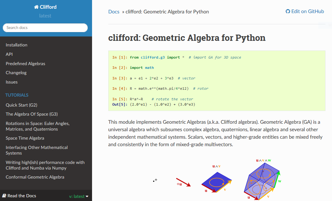
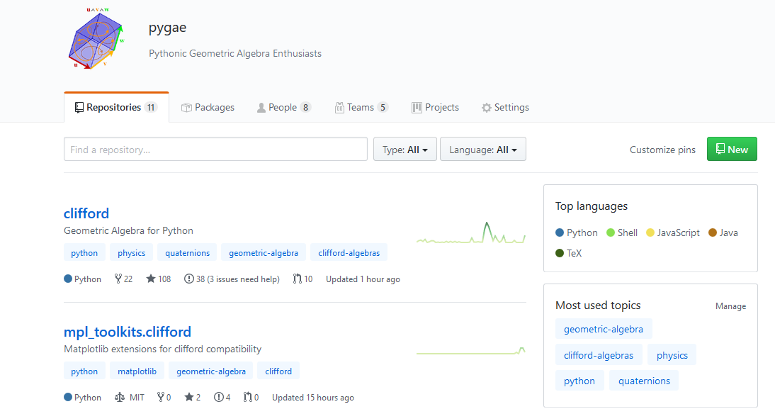
If you are interested in getting involved then check out the pygae github group and have a go with the python clifford package for numerical GA
Event Horizon Telescope Collaboration
Let's get started
Rosquist, K. (2013).Modelling and Control of a Parallel Kinematic Robot. ISRNLUTFD2/TFRT–5929–SE. Master’s Thesis. Department of Automatic Control,LTH, Lund University, Lund, Sweden
H. Hadfield and J. Lasenby, ‘Direct Linear Interpolation of Geometric Objects in Conformal Geometric Algebra’, Advances in Applied Clifford Algebras 29, no. 4 (September 2019): 85, https://doi.org/10.1007/s00006-019-1003-y.
Anthony Lasenby, Robert Lasenby, and Chris Doran, ‘Rigid Body Dynamics and Conformal Geometric Algebra’, in Guide to Geometric Algebra in Practice, ed. Leo Dorst and Joan Lasenby (London: Springer, 2011), 3–24, https://doi.org/10.1007/978-0-85729-811-9_1.
Jaime Gallardo-Alvarado, Kinematic Analysis of Parallel Manipulators by Algebraic Screw Theory (Springer International Publishing, 2016), https://doi.org/10.1007/978-3-319-31126-5.
Tischler, C.R., Downing, D.M., Lucas, S.R., Martins, D.: Rigid-body inertia and screw geometry. In: Proceedings of a symposium commemorating the legacy, works, and life of Sir Robert Stawell Ball upon the 100th anniversary of a treatise on the theory of screws. Cambridge (2000)
Michael Boyle, ‘The Integration of Angular Velocity’, Advances in Applied Clifford Algebras 27, no. 3 (1 September 2017): 2345–74, https://doi.org/10.1007/s00006-017-0793-z.
By Hugo Hadfield
GAME2020: Robots, Ganja and Screw Theory. This is the presentation that accompanies my talk at GAME2020 (video here: https://www.youtube.com/watch?v=j2x_TG8E3_k&t=5s ). The presentation covers the forward and inverse kinematics of serial and parallel robots, embedding screw theory into geometric algebra and simulating rigid body dynamics with this framework.


