Honeycomb Geometry
Rigid Motions on the Hexagonal Grid

The figure comes from "Insects The Yearbook of Agriculture 1952" United States Dept. of Agriculture." Published by the US Government Printing Office. Deemed to be in the Public Domain under US Law.
by Kacper Pluta, Pascal Romon, Yukiko Kenmochi and Nicolas Passat
Motivations
Digitized rigid motions defined on the square grid are burdened with an incompatibility between rotations and the geometry of the grid.
Agenda
-
Introduction to the Bees' Point of View
-
Quick Introduction to Rigid Motions
- Neighborhood Motion Maps
- Contributions
- Conclusions & Perspectives
The beehive figure's source and author unknown (if you recognize it, please let me know). The image of the bee comes from http://karenswhimsy.com/public-domain-images (public domain)
Introduction to the Bees' Point of View
Or why bees are right
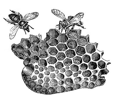
The figure comes from http://thegraphicsfairy.com/vintage-clip-art-bees-with-honeycomb
Square grid
+ Memory addressing
+ Sampling is easy to define
Hexagonal grid
+ Uniform connectivity
+ Equidistant neighbors
+ Sampling is optimal
- Sampling is not optimal (ask bees)
- Neighbors are not equidistant
- Connectivity paradox
- Memory addressing is not trivial
- Sampling is difficult to define
Pros and Cons
Square grid
+ Memory addressing
+ Sampling is easy to define
Hexagonal grid
+ Uniform connectivity
+ Equidistant neighbors
+ Sampling is optimal
~ Memory addressing is not trivial
~ Sampling is difficult to define
Pros and Cons
- Sampling is not optimal (ask bees)
- Neighbors are not equidistant
~ Connectivity paradox
Hexagonal Grid


\Lambda = \mathbb{Z}\epsilon_1 \oplus \mathbb{Z}\epsilon_2
The hexagonal lattice:
and the hexagonal grid
\mathcal{H}
The figure by Pearson Scott Foresman, Wikimedia.
Digitization Model

The digitization cell of
\kappa
denoted by
\mathcal{C}(\kappa).
Digitization Model
The digitization operator is defined as
\mathcal{D}: \mathbb{R}^2 \rightarrow \Lambda
such that
\forall \mathbf{x} \in \mathbb{R}^2, \exists! \mathcal{D}(\mathbf{x}) \in \Lambda
\mathbf{x} \in \mathcal{C}(\mathcal{D}(\mathbf{x})).
and
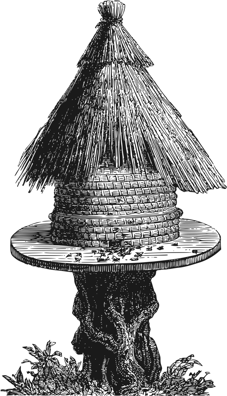
Quick Lesson on Rigid Motions
Or how to become a beekeeper. Part I - Equipment
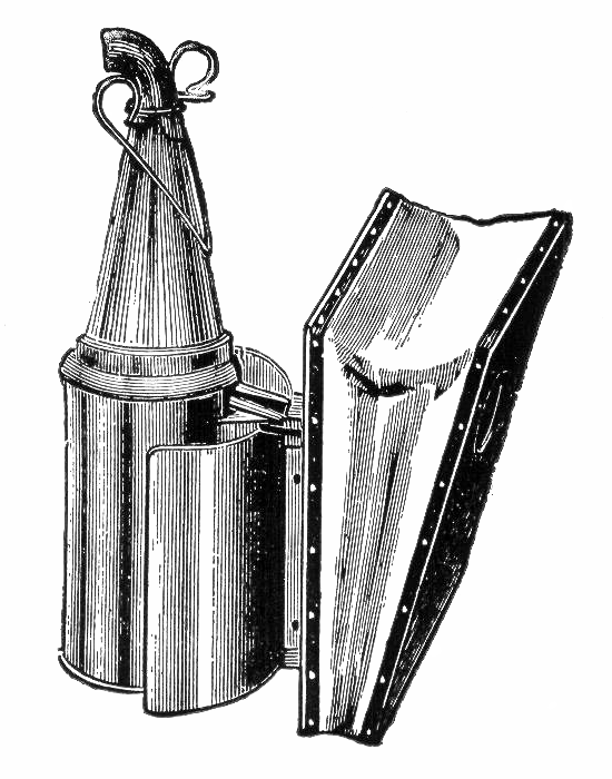
The figure comes from Wikimedia. Original source The New Student's Reference Work (public domain)
\left|
\begin{array}{lllll}
\mathcal{U} & : & \mathbb{R}^2 & \to & \mathbb{R}^2 \\
& & \mathbf{x} & \mapsto & \mathbf{R} \mathbf{x} + \mathbf{t}
\end{array}
\right.
Rigid Motions on
\mathbb{R}^2
Properties
-
Isometry
-
Bijective
\mathbf{R}
- rotation matrix
\mathbf{t}
- translation vector
U = \mathcal{D}\ \circ \mathcal{U}_{|\Lambda}
\Lambda
Properties
- Non-injective


- Non-surjective
- Do not preserve distances
\mathcal{U}(\Lambda)
Rigid Motions on
Related Studies
- Nouvel, B., Rémila, E.: On colorations induced by discrete rotations. In: DGCI, Proceedings. Volume 2886 of Lecture Notes in Computer Science., Springer (2003) 174–183
- Pluta, K., Romon, P., Kenmochi, Y., Passat, N.: Bijective digitized rigid motions on subsets of the plane. Journal of Mathematical Imaging and Vision (2017)
Contributions in Short
- Extension of the former framework to the hexagonal grid
- Comparison of the loss of information between the hexagonal and square grids
- Complete set of neighborhood motion maps
- Source code of a tool to study digitized rigid motions on the hexagonal grid
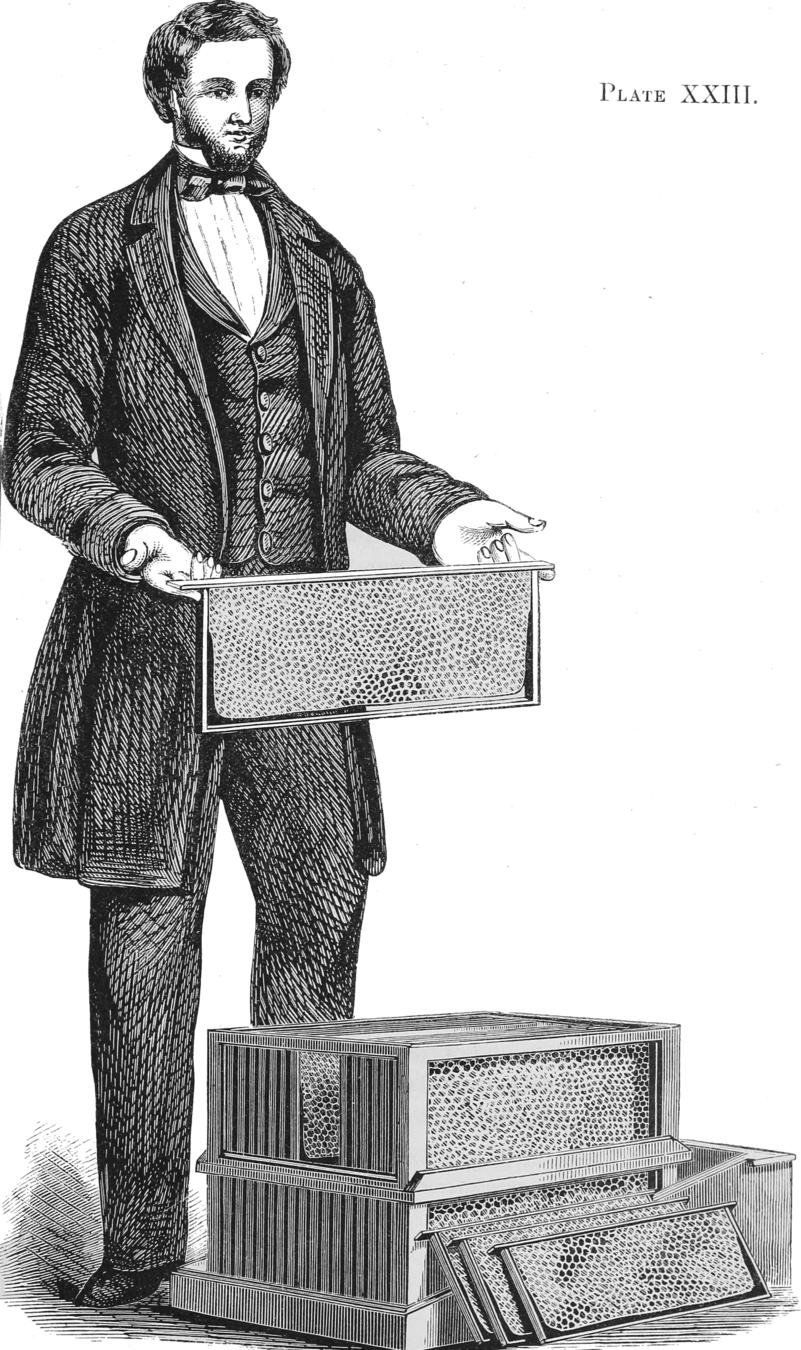
Pure extracted honey
Neighborhood Motion Maps
Or a manual of instructions in apiculture

The figure comes from Wikimedia. The original source The honey bee: a manual of instruction in apiculture (public domain)
Neighborhood

The neighborhood of
\kappa \in \Lambda
(of squared radius
r \in \mathbb{R}_+
):
\mathcal{N}_r(\kappa) = \big\{ \kappa + \delta \in \Lambda \mid \|\delta \|^2 \leq r \big\}
Neighborhood Motion Maps
The neighborhood motion map of
\kappa \in \Lambda
for given a rigid motion
r \in \mathbb{R}_+
U
and
\left|
\begin{array}{lllll}
\mathcal{G}^U_r & : & \mathcal{N}_r(0) & \to & \mathcal{N}_{r'}(0) \\
& & \delta & \mapsto & U(\kappa + \delta) - U(\kappa).
\end{array}
\right.


Remainder Map step-by-step

\kappa
Remainder Map step-by-step

\mathcal{U}(\kappa + \delta) =
\mathbf{R}\delta
+ \mathcal{U}(\kappa)
\mathcal{U}(\kappa + \delta)
Remainder Map step-by-step
Without loss of generality,
U(\kappa)
is the origin, and then
\mathcal{U}(\delta) = \mathbf{R}\delta + \mathcal{U}(\kappa) - U(\kappa)
\mathbf{R}\delta
\delta
\mathcal{U}(\kappa) - U(\kappa)
Remainder Map step-by-step
The remainder map defined as
\mathcal{F}(\kappa) = \mathcal{U}(\kappa) - U(\kappa) \in \mathcal{C}(\mathbf{0})
where the range
\mathcal{C}(\mathbf{0})
is called the remainder range.
\mathcal{F}(\kappa) = \mathcal{U}(\kappa) - U(\kappa)

Remainder Map and Critical Rigid Motions

Remainder Map and Critical Rigid Motions

Such critical cases can be observed via the relative positions of ,
\mathcal{F}(\kappa)
\mathcal{H} - \mathbf{R}\delta
That is to say
\mathcal{C}(\mathbf{0}) \cap (\mathcal{H} - \mathbf{R}\delta).
and are formulated as the translation .
Remainder Map and Critical Rigid Motions
\mathcal{H} - \mathbf{R}\delta
Critical line segments

\mathscr{H} = \bigcup \limits_{\delta \in \mathcal{N}_r(\mathbf{0})} (\mathcal{H} - \mathbf{R}\delta) \cap \mathcal{C}(\mathbf{0})
Frames
Each region bounded by the critical line segments is called a frame.

Frames
For any
\kappa, \lambda \in \Lambda, \mathcal{G}^U_r(\kappa) = \mathcal{G}^U_r(\lambda)
if and only if
\mathcal{F}(\kappa)
and
\mathcal{F}(\lambda)
are in the same frame.
Proposition
Remainder Range Partitioning


At most 49 frames per partitioning.
Contributions
Or extracting the pure, organic honey
The figure comes from Wikimedia. The original comes from A practical treatise on the hive and honey-bee (public domain)


Non-injective Digitized Rigid Motions

\mathcal{F}(\Lambda)
For what kind of parameters has the remainder map a finite number of images?
Eisenstein Rational Rotations
Eisenstein Rational Rotations
\mathcal{F}(\Lambda)
If
\cos\theta = \frac{2a -b}{2 c}
and
\sin\theta = \frac{\sqrt{3}b}{2 c}
where
(a,b,c)\in \mathbb{Z}^3, \gcd(a,b,c) = 1
and
0 < a < c < b,
Corollary
then the remainder map has a finite number
of images.
Loss of Information

Conclusions & Perspectives
- An extension of a framework to study digitized rigid motions
- Characterization of rational rotations
- We have showed that the loss of information is relatively lower for digitized rigid motions defined on the hexagonal grid
- Our tools on BSD-3 license: https://github.com/copyme/NeighborhoodMotionMapsTools

hal.archives-ouvertes.fr/hal-01540772
Homework
If you want to get into the honey business, then this book is an obligatory lecture: Middleton, Lee, and Jayanthi Sivaswamy. Hexagonal image processing: A practical approach. Springer Science & Business Media, 2006.
Honeycomb Geometry: Rigid Motions on the Hexagonal Grid
By Kacper Pluta
Honeycomb Geometry: Rigid Motions on the Hexagonal Grid
Presentation of a paper under the same name. The presentation was presented during DGCI17 (Vienna).


