Geometric hydrodynamics in

Klas Modin

Topics

  • Motion of ideal fluids
  • Arnold's geometric insight
  • What's special about flatland?
  • Yudovich's existence result
  • Onsager's statistical hydrodynamics
  • Long-time problem of long-time behavior
  • Quantization and Zeitlin's model

Geometry of the Euler equations

\dot v + \nabla_v v = -\nabla p
\operatorname{div}v = 0

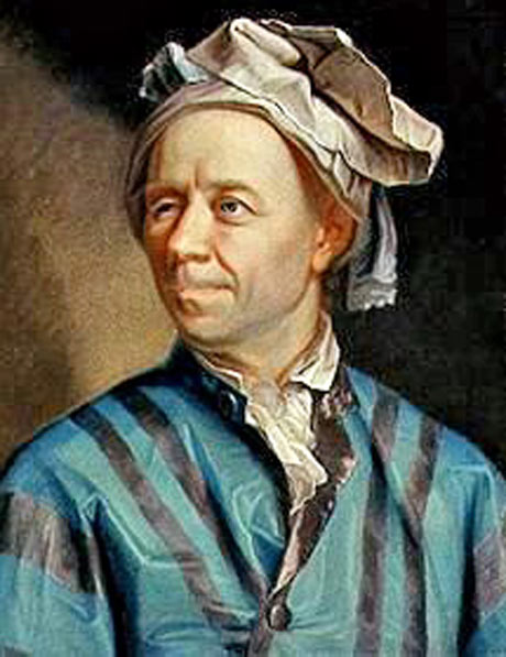
Euler's equations describe Riemannian geodesics on

\operatorname{Diff}_{\mu}(M) = \{ \varphi\in\operatorname{Diff}(M) \mid |D\varphi| = 1 \}

But how?

Riemannian metrics on Lie groups

V \in T_g G
g
\langle V,V\rangle_g =
?
G

Riemannian metrics on Lie groups

V\cdot g^{-1} \in \mathfrak{g}
e
\langle V,V\rangle_g =
\langle V\cdot g^{-1},V\cdot g^{-1}\rangle_e
G

"Right-invariant" Riemannian metric determined by inner product on \(\mathfrak{g}\)

Governing equations

\mathfrak{g}^*
TG
G
\displaystyle\frac{d}{dt}\frac{\partial L}{\partial \dot g} = \frac{\partial L}{\partial g}

\(G\)

\(T_eG\simeq\mathfrak g\)

L(g,\dot g) = \langle\dot g,\dot g\rangle_g
\displaystyle \dot m = \mathrm{ad}^*_v m
\displaystyle \dot g = v\cdot g
\displaystyle \mathrm{Ad}^*_g m_0 = \langle v,\cdot \rangle
\displaystyle m = \langle v,\cdot \rangle

Euler-Arnold

(Lie-Poisson)

Euler-Lagrange

Yudovich

Simple example: free rigid body

G = SO(3), \quad \mathfrak{g} = \mathfrak{so}(3)\simeq \mathbb{R}^3

Inner product: moments of inertia tensor \(\mathbb{I}\)

\displaystyle \dot m = \underbrace{(\mathbb{I}^{-1} m)}_{v}\times m
\mathrm{ad}^*_v m = v\times m

Arnold's example: Euler equations

G = \operatorname{Diff}_\mu(M), \quad \mathfrak{g} = \mathfrak{X}_\mu(M) = \{ v\mid \operatorname{div}v=0 \}

Inner product:

\displaystyle\langle v,v\rangle_{L^2} = \int_M \lvert v \rvert^2 \mu

Arnold's theorem:  \(\gamma(t)\in \operatorname{Diff}_\mu(M)\) geodesic curve \(\Rightarrow\) vector field \(v(t) = \dot\gamma(t)\circ\gamma(t)^{-1}\) fulfills Euler's equations

But in what sense is \(\operatorname{Diff}_\mu(M)\) a Lie group?

Manifold structure of \(\operatorname{Diff}^s(M)\)

\operatorname{Diff}^s(M)
U \subset H^s
V \subset H^s

Thm [Palais, Omori, Ebin, Ebin and Marsden] 

\(\operatorname{Diff}^s(M)\) is smooth Hilbert manifold if \(s>\operatorname{dim}(M)/2+1\)

\(\operatorname{Diff}^s_\mu(M)\) is a submanifold

What about Lie group structure?

Thm [Ebin] 

\(\operatorname{Diff}^s(M)\) topological group if \(s>\operatorname{dim}(M)/2+1\)

Group structure:

(\varphi,\eta)\mapsto \varphi\circ \eta
\varphi\mapsto \varphi^{-1}

Failure of smoothness (illustration):
Compute  derivative of left translation \(L_\varphi(\eta) = \varphi\circ\eta\)

T_\eta L_\varphi\cdot V = D\varphi\circ\eta \cdot V
H^s

What about Lie group structure?

Thm [Ebin] 

\(\operatorname{Diff}^s(M)\) topological group if \(s>\operatorname{dim}(M)/2+1\)

Group structure:

(\varphi,\eta)\mapsto \varphi\circ \eta
\varphi\mapsto \varphi^{-1}

Failure of smoothness (illustration):
Compute  derivative of left translation \(L_\varphi(\eta) = \varphi\circ\eta\)

T_\eta L_\varphi\cdot V = D\varphi\circ\eta \cdot V
H^{s-1}

"Fix" the Lie group structure

Option 1

\operatorname{Diff}(M)
U \subset C^\infty
V \subset C^\infty

Use Fréchet manifolds instead

  • Pros: proper Lie group structure
  • Cons: no Picard iterations

Option 2

Right translation \(R_\varphi(\eta) = \eta\circ\varphi\)

T_\eta R_\varphi\cdot V = V\circ\varphi
H^s

So, let's work only with right translation

Crazy idea, but it works!

Simple example of how it works

\dot v - \dot v_{xx} + 3 v v_x - 2v_x v_{xx} - v v_{xxx} = 0

Camassa-Holm equation

A \dot v + v Av_x + 2 v_x A v = 0,
A = 1 - \partial_{xx}^2
v(t,\cdot) \in H^s(S^1), \quad s>2

Why PDE not ODE?

Idea: [Ebin and Marsden] maybe geodesic equation on \(T\operatorname{Diff}^s(S^1)\) is an ODE

H^{s-2}
H^{s-2}
H^{s-3}

Camassa-Holm as geodesic equation

\operatorname{Diff}^s(S^1)
H^s(S^1)
v(t)
H^s(S^1) \ni v(t) \mapsto (\underbrace{v(t)\circ\varphi(t)}_{\dot\varphi(t)},\varphi(t))\in T\operatorname{Diff}^s(S^1)
\dot\varphi(t) = v(t)\circ\varphi(t)

Camassa-Holm as geodesic equation

\operatorname{Diff}^s(S^1)
H^s(S^1)
\dot\varphi(t)
H^s(S^1) \ni v(t) \mapsto (\underbrace{v(t)\circ\varphi(t)}_{\dot\varphi(t)},\varphi(t))\in T\operatorname{Diff}^s(S^1)
\dot\varphi(t) = v(t)\circ\varphi(t)
\ddot\varphi = \dot v\circ\varphi + v_x\circ\varphi \, \dot\varphi
= (\dot v + v_x v)\circ\varphi = \Big( A^{-1}(-v Av_x - 2 v_x A v + A(v_x v)) \Big)\circ\varphi
= \Big( A^{-1}(-v Av_x + v A v_x + H^{s-2}\text{-terms}) \Big)\circ\varphi

Camassa-Holm as geodesic equation

\operatorname{Diff}^s(S^1)
H^s(S^1)
\dot\varphi(t)
\dot\varphi(t) = v(t)\circ\varphi(t)
\ddot\varphi = \dot v\circ\varphi + v_x\circ\varphi \, \dot\varphi
= (\dot v + v_x v)\circ\varphi = \Big( A^{-1}(-v Av_x - 2 v_x A v + A(v_x v)) \Big)\circ\varphi
= \Big( A^{-1}(-v Av_x + v A v_x + H^{s-2}\text{-terms}) \Big)\circ\varphi

Are we done?

No! RHS must be smooth as function of \( \varphi,\dot\varphi\) but \(v=\dot\varphi\circ\varphi^{-1}\)

\underbrace{\phantom{gffdffd}}_{B(v,v)}

Second piece of magic

\ddot\varphi = \tilde A^{-1}_\varphi (\tilde B_\varphi(\dot\varphi,\dot\varphi)), \quad B:H^s \times H^s\to H^{s-2}
P: H^s \to H^{s-2}, \; \tilde P_\varphi: T_\varphi\operatorname{Diff}^s(S^1)\to T^{s-2}_\varphi\operatorname{Diff}^s(S^1)
\tilde P_\varphi V = (P(V\circ\varphi^{-1}))\circ\varphi

Geodesic equation, again

Lemma: Mapping \(T\operatorname{Diff}^s(S^1)\to T^{s-1}\operatorname{Diff}^s(S^1)\) given by \[(\varphi,\dot\varphi)\mapsto (\partial_x(\dot\varphi\circ\varphi^{-1}))\circ\varphi \] is smooth

Second piece of magic

\ddot\varphi = \tilde A^{-1}_\varphi (\tilde B_\varphi(\dot\varphi,\dot\varphi)), \quad B:H^s \times H^s\to H^{s-2}

Geodesic equation, again

Lemma: Mapping \(T\operatorname{Diff}^s(S^1)\to T^{s-1}\operatorname{Diff}^s(S^1)\) given by \[(\varphi,\dot\varphi)\mapsto (\partial_x(\dot\varphi\circ\varphi^{-1}))\circ\varphi \] is smooth

Proof:

\displaystyle (\partial_x (\dot\varphi\circ\varphi^{-1}))\circ\varphi = \dot\varphi_x((\partial_x\varphi^{-1})\circ\varphi) = \frac{\dot\varphi_x}{\varphi_x}

Second piece of magic

\ddot\varphi = \tilde A^{-1}_\varphi (\tilde B_\varphi(\dot\varphi,\dot\varphi)), \quad B:H^s \times H^s\to H^{s-2}

Geodesic equation, again

Lemma: Mapping \(T\operatorname{Diff}^s(S^1)\to T^{s-1}\operatorname{Diff}^s(S^1)\) given by \[(\varphi,\dot\varphi)\mapsto (\partial_x(\dot\varphi\circ\varphi^{-1}))\circ\varphi \] is smooth

Thm: Spray \(T\operatorname{Diff}^s(S^1)\to T^{s-2}\operatorname{Diff}^s(S^1)\) given by \[(\varphi,\dot\varphi)\mapsto \tilde A^{-1}_\varphi (\tilde B_\varphi(\dot\varphi,\dot\varphi)) \] is smooth

That's it!

Another case: symplectomorphisms

G = \operatorname{Diff}_\Omega(M), \quad \mathfrak{g} = \mathfrak{X}_\Omega(M) = \{ v\mid L_v\Omega=0 \}

\((M,\Omega)\) symplectic

\(v=X_\psi\) for Hamiltonian \(\psi\)

Change of coordinates: \( \psi \leftrightarrow X_\psi\)

Lie bracket
Kinetic energy
[\cdot,\cdot]
v \in \mathfrak{X}_\Omega(M)
\psi\in C^\infty(M)
\{\cdot,\cdot\}
\int_M |v|^2
\int_M \psi(-\Delta)^{-1}\psi

\(L^2\)

\(H^{-1}\)

?

?

E-A equation for \(\mathfrak{g} = C^\infty(M)\)

\dot\omega =-\{\psi,\omega \}
-\Delta\psi = \omega
\dot\omega + v\cdot \nabla\omega = 0

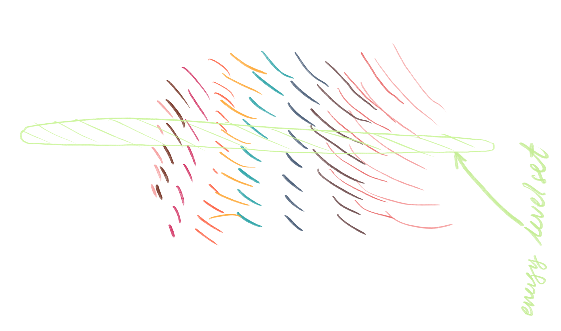
level-sets of \(\omega\)

Restriction to smooth dual: \(C^\infty(M)\subset\mathfrak{g}^*\) via \(L^2\) pairing

\langle \mathrm{ad}^*_\psi\omega,\xi\rangle_{L^2} = \langle \omega, \{\psi,\xi \}\rangle_{L^2} = \{-\{\psi,\omega \},\xi \}_{L^2}

Casimir functions: \( \mathcal C_f(\omega) = \int_{S^2}f(\omega)\)

Finite-dim (weak) orbits: \(\omega = \sum_{k=1}^N \Gamma_k \delta_{x_k} \)

Comparison

\operatorname{Diff}_\mu(M)
\operatorname{Diff}_\Omega(M)\subseteq \operatorname{Diff}_{\Omega^n}(M)
  • volume-preserving flow
  • transport of vorticity 2-form \(\beta = dv^\flat\)
  • Casimirs:
    only helicity (in 3-D)
  • symplectic flow
  • transport of vorticity function \(\omega = \operatorname{curl}v\)
  • Casimirs:
    infinitely many

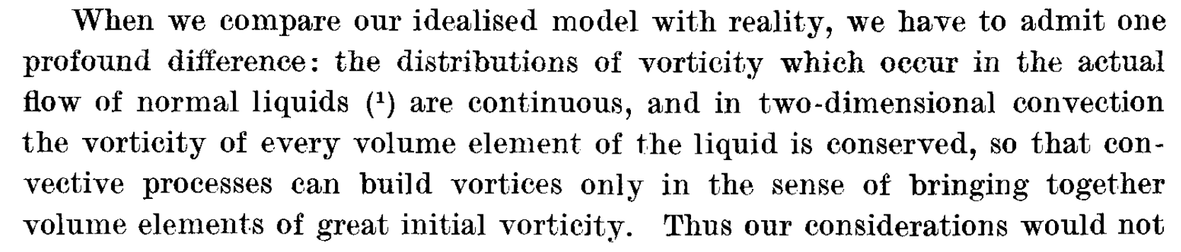
Consequence: 2-D Euler richer geometric structure than 3-D

\Rightarrow
  • global existence
  • inverse energy cascade
  • vortex condensation

Yudovich's existence result

Yudovich formulation:

\dot\Phi = X_\psi\circ\Phi, \quad \Delta\psi = \omega_0\circ\Phi^{-1}

Vorticity formulation:

\dot\omega = \{\psi,\omega \}, \quad \Delta\psi = \omega

Yudovich is weaker: \(\omega_0 \in L^\infty\) enough

Fixed-point iteration over \(v,\Phi,\omega\):

\frac{\partial}{\partial t}\Phi^{n}(x,t) = v^{n-1}(\Phi^n(x,t), t)
v^n = X_{\Delta^{-1}\omega^{n-1}}
\omega^n(x,t) = \omega_0(\Phi^n(x,-t))
\Rightarrow

\(L^\infty\) global existence

Generic long-time behavior?

Statistical mechanics

for 2-D Euler

Idea by Onsager (1949):

  • Approximate \(\omega\) by PV for large \(N\)
  • Find invariant measure and presume ergodicity

Hamiltonian function:

\displaystyle H(x_1,\ldots,x_N) = \sum_{kl} \Gamma_k\Gamma_l G(x_1, x_N)

Statistical mechanics

for 2-D Euler

Idea by Onsager (1949):

  • Approximate \(\omega\) by PV for large \(N\)
  • Find invariant measure and presume ergodicity

Hamiltonian function:

\displaystyle H(x_1,\ldots,x_N) = -\sum_{kl} \Gamma_k\Gamma_l \log |x_1-x_N|

Onsager's observation:

Pos. and neg. strengths \(\Rightarrow\) energy takes values \(-\infty\) to \(\infty\)

\(\Rightarrow\) phase volume function \(\mathrm{vol}(E)\) has inflection point

Statistical mechanics

for 2-D Euler

Idea by Onsager (1949):

  • Approximate \(\omega\) by PV for large \(N\)
  • Find invariant measure and presume ergodicity

Hamiltonian function:

\displaystyle H(x_1,\ldots,x_N) = -\sum \Gamma_k\Gamma_l \log |x_1-x_N|

Problems with Onsager's theory

  • PV solutions far from smooth (\(H^{-1}\) but never \(L^p\))
  • \(\Rightarrow\) No Casimir functions
  • But experiments and numerical simulations strongly indicate that Casimirs affect long-time behavior

Numerical experiments contradict statistical theories

Numerical experiments contradict statistical theories

Alignment with

point-vortex dynamics

Mechanism for long-time behaviour

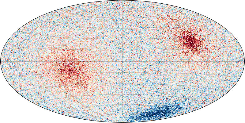
Observation: large scale motion quasiperiodic

Assumptions for new mechanism:

  1. Small formations merge to larger (inverse energy cascade)
  2. Well-separated blobs interact approximately by PVD
  3. Dynamics is not integrable \(\Rightarrow\) blobs continue to merge
  4. \(k\)-PVD integrable \(\Rightarrow\) quasi-periodicity prevents further mixing

Jewel of 2-D turbulence

For "generic" \(\omega_0\), what is the typical long-time behaviour?

More precise (Shnirelman 1993):

\displaystyle\Omega_+(\omega_0) = \bigcap_{s\geq 0}\overline{\{\Phi_t(\omega_0)\mid t\geq s \}}^*

What is contained in \(\Omega_+(\omega_0)\) ?

Related (Sverak 2011): generic trajectories

\{\Phi_t(\omega_0)\mid t\in \mathbb{R} \}

are not \(L^2\) precompact   ( \(\simeq\) enstrophy cascade )

Structure preserving discretization via quantization

Vladimir Zeitlin

Classical

Quantized

\omega \in C^\infty
W \in \mathfrak{su}(N)
\{\cdot,\cdot \}
\frac{1}{\hbar}[\cdot,\cdot ]
\dot\omega = \{\psi,\omega \}
\dot W = \frac{1}{\hbar}[P,W]

Discrete Laplace-Beltrami on \(\mathfrak{su}(N)\)

  • Hoppe & Yau, 1998
    \[\Delta_N W =\frac{N^2-1}{2}\sum_{i=1}^3[X_i^N,[X_i^N,W]]\]
\displaystyle\dot W = \frac{1}{\hbar}[\Delta_N^{-1}W,W]

What is \(\Delta_N\) and how to compute \(\Delta_N^{-1}W\) ?


  • \(\Delta_N\) admits sparse \(LU\)-factorization

Spatial discretization obtained!

\displaystyle \dot W = \frac{1}{\hbar}[\Delta_N^{-1}W,W]

Note: corresponds to

\(N^2\) spherical harmonics

\(O(N^2)\) operations

\(O(N^3)\) operations

Isospectral flow \(\Rightarrow\) discrete Casimirs

\displaystyle C^N_f(W) = \operatorname{tr}(f(W))

Geometric hydrodynamics in Flatland

By Klas Modin

Geometric hydrodynamics in Flatland

Mini-course given in Santiago de Compostela in September 2023.

  • 166