Legislative Bargaining

Lecture 5, Political Economics I

OSIPP, Osaka University

17 November, 2017

Masa Kudamatsu

Motivation #1

The models we have discussed so far in this course

Many elected politicians negotiate with each other to enact policies

The single elected politician can unilaterally implement policies

In reality

e.g. Fiscal budget has to be approved by legislature

The legislative bargaining model

is a framework to analyze such collective decision-making

Motivation #2

The legislative bargaining model

is another way to pin down an equilibrium policy in such cases

For policy issues where there is no median voter (cf. Lecture 1)

e.g. The division-of-a-pie problem

We need a model that allows us to find an equilibrium

e.g. Probabilistic Voting Model (cf. Lecture 3)

Motivation #3

The legislative bargaining model is an extension to allow

(1) multiple players

(2) majority voting, rather than unanimity

In game theory

The Rubinstein bargaining game is a framework

to analyze the negotiation between two persons

Basic Model

with one-dimensional policy space

Originally proposed by Baron and Ferejohn (1989)

Here we follow Section 5.4 of Persson and Tabellini (2000)

Players

Three legislators, $J \in \{L,M,R\}$

Think of each as a citizen-candidate elected in each constituency

Endowments

Each legislator $J$ is endowed with income $y^J$ with $y^L<y^M<y^R$

Preference

W^J(g) = (1-\tau)y^J+H(g)

W^J(g) = (1-\tau)y^J+H(g)

Government budget constraint

\tau y = g

\tau y = g

where $y$ is per capita income w/ pop size 1

Each legislator's bliss point

g^J =\arg\max_g W^J(g) = (1-\frac{g}{y})y^J+H(g)

g^J =\arg\max_g W^J(g) = (1-\frac{g}{y})y^J+H(g)

Government budget constraint

\tau y = g

\tau y = g

where $y$ is per capita income w/ pop size 1

Preference

W^J(g) = (1-\tau)y^J+H(g)

W^J(g) = (1-\tau)y^J+H(g)

Plugging the budget constraint into legislator J's preference...

Each legislator's bliss point

g^J =\arg\max_g W^J(g) = (1-\frac{g}{y})y^J+H(g)

g^J =\arg\max_g W^J(g) = (1-\frac{g}{y})y^J+H(g)

First order condition yields:

H_g(g^J)=\frac{y^J}{y}

H_g(g^J)=\frac{y^J}{y}

Each legislator's bliss point

g^J =\arg\max_g W^J(g) = (1-\frac{g}{y})y^J+H(g)

g^J =\arg\max_g W^J(g) = (1-\frac{g}{y})y^J+H(g)

First order condition yields:

H_g(g^J)=\frac{y^J}{y}

H_g(g^J)=\frac{y^J}{y}

g

H_g(g)

H_g(g)

y^R/y

y^R/y

y^M/y

y^M/y

y^L/y

y^L/y

g^R

g^R

g^M

g^M

g^L

g^L

g^R< g^M< g^L

g^R< g^M< g^L

So we have:

Timing of Events

Nature picks $J \in \{R,M,L\}$ as the agenda setter

Denote this legislator by $A$

Legislator $A$ proposes $g_A$

All legislators vote on the proposal $g_A$

If at least two parties vote yes, $g_A$ will be implemented

Otherwise, the default policy, $\bar{g}$, will be implemented

"Agenda setter" in reality

Cabinet ministers in parliamentary systems (UK, etc.)

Legislative committees in presidential systems (US etc.)

Agriculture Appropriations Armed Services Budget

Education and the Workforce Energy and Commerce Ethics

Financial Services Foreign Affairs Homeland Security

House Administration Judiciary Natural Resources

Oversight and Government Reform Rules

Science, Space, and Technology Small Business

Transportation and Infrastructure Veterans' Affairs Ways and Means

Source: www.congress.gov/committees

Committees in U.S. Lower House

We will see this committee in action later

Default policy in reality #1

Government shutdown in U.S.

October 1st-16th, 2013

Due to the deadlock between the Republican-controlled House

and the Democrat-controlled Senate over Obamacare

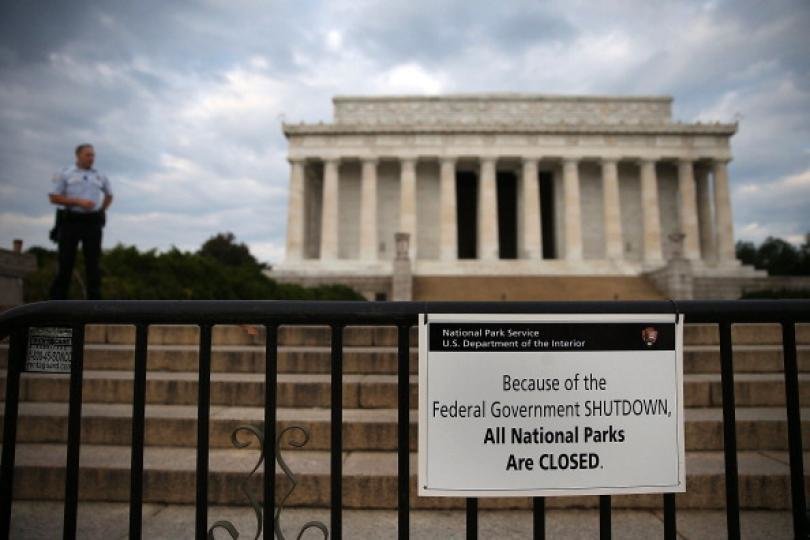
Image source: www.ibtimes.com/government-shutdown-2013-impact-national-parks-museums-us-travel-1413078

Most recent case:

Default policy in reality #2

e.g. Art. 312 of Treaty on the Functioning of the European Union

Where no Council regulation determining a new financial framework has been adopted by the end of the previous financial framework, the ceilings and other provisions corresponding to the last year of that framework shall be extended until such time as that act is adopted.

(Quoted by Piguillem and Riboni (2015), footnote 8)

The policy adopted in the previous fiscal year

Default policy in reality #1

Government shutdown in U.S.

October 1st-16th, 2013

Due to the deadlock between the Republican-controlled House

and the Democrat-controlled Senate over Obamacare

Image source: www.ibtimes.com/government-shutdown-2013-impact-national-parks-museums-us-travel-1413078

Most recent case:

Analysis

Backward induction

Nature picks $J \in \{R,M,L\}$ as the agenda setter

Denote this legislator by $A$

Legislator $A$ proposes $g_A$

All legislators vote on the proposal $g_A$

If at least two parties vote yes, $g_A$ will be implemented

Otherwise, the default policy, $\bar{g}$, will be implemented

Backward induction

Legislators $J \neq A$ vote yes to $g_A$ as long as

W^J(g_A) \geq W^J(\bar{g})

W^J(g_A) \geq W^J(\bar{g})

Since $W^J(g)$ is single-peaked, this means

Backward induction

Legislators $J \neq A$ vote yes to $g_A$ as long as

W^J(g_A) \geq W^J(\bar{g})

W^J(g_A) \geq W^J(\bar{g})

Since $W^J(g)$ is single-peaked, this means

g^J

g^J

\bar{g}

\bar{g}

W_J^{-1}(W^J(\bar{g}))

W_J^{-1}(W^J(\bar{g}))

g_A

g_A

Accept

Backward induction

Nature picks $J \in \{R,M,L\}$ as the agenda setter

Denote this legislator by $A$

Legislator $A$ proposes $g_A$

All legislators vote on the proposal $g_A$

If at least two parties vote yes, $g_A$ will be implemented

Otherwise, the default policy, $\bar{g}$, will be implemented

Case 1: Legislator M as the agenda setter

g^M

g^M

g^R

g^R

g^L

g^L

g_A

g_A

Case 1: Legislator M as the agenda setter (cont.)

g^M

g^M

g^R

g^R

g^L

g^L

g_A

g_A

Suppose

\bar{g}

\bar{g}

\bar{g} < g^M

\bar{g} < g^M

Case 1: Legislator M as the agenda setter (cont.)

g^M

g^M

g^R

g^R

g^L

g^L

g_A

g_A

Suppose

\bar{g}

\bar{g}

\bar{g} < g^M

\bar{g} < g^M

Legislator R will vote yes if

g_A \leq \bar{g}

g_A \leq \bar{g}

Case 1: Legislator M as the agenda setter (cont.)

g^M

g^M

g^R

g^R

g^L

g^L

g_A

g_A

Suppose

\bar{g}

\bar{g}

\bar{g} < g^M

\bar{g} < g^M

Legislator L will vote yes if

g_A \geq \bar{g}

g_A \geq \bar{g}

Legislator M's bliss point $g^M$ will be accepted by L

It's optimal to propose $g_A = g^M$

Case 1: Legislator M as the agenda setter (cont.)

g^M

g^M

g^R

g^R

g^L

g^L

g_A

g_A

Suppose

\bar{g}

\bar{g}

\bar{g} > g^M

\bar{g} > g^M

Case 1: Legislator M as the agenda setter (cont.)

g^M

g^M

g^R

g^R

g^L

g^L

g_A

g_A

Legislator L will vote yes if

g_A \geq \bar{g}

g_A \geq \bar{g}

Suppose

\bar{g} > g^M

\bar{g} > g^M

\bar{g}

\bar{g}

Case 1: Legislator M as the agenda setter (cont.)

g^M

g^M

g^R

g^R

g^L

g^L

g_A

g_A

Legislator R will vote yes if

g_A \leq \bar{g}

g_A \leq \bar{g}

Suppose

\bar{g} > g^M

\bar{g} > g^M

\bar{g}

\bar{g}

Legislator M's bliss point $g^M$ will be accepted by R

It's optimal to propose $g_A = g^M$

Case 1: Legislator M as the agenda setter (cont.)

g^M

g^M

g^R

g^R

g^L

g^L

g_A

g_A

For all $\bar{g}$,

Legislator M proposes $g_A = g^M$

Then

R votes in favor if $\bar{g} > g^M $

L votes in favor otherwise

So far the prediction is the same as the median voter theorem

Case 2: Legislator L as the agenda setter

g^M

g^M

g^R

g^R

g^L

g^L

g_A

g_A

Case 2: Legislator L as the agenda setter

g^M

g^M

g^R

g^R

g^L

g^L

g_A

g_A

Suppose

\bar{g}

\bar{g}

\bar{g} \geq g^L

\bar{g} \geq g^L

Case 2: Legislator L as the agenda setter

g^M

g^M

g^R

g^R

g^L

g^L

g_A

g_A

Suppose

\bar{g}

\bar{g}

Legislator R will vote yes if

g_A \leq \bar{g}

g_A \leq \bar{g}

\bar{g} \geq g^L

\bar{g} \geq g^L

Case 2: Legislator L as the agenda setter

g^M

g^M

g^R

g^R

g^L

g^L

g_A

g_A

Suppose

\bar{g}

\bar{g}

Legislator M will vote yes if

W_M^{-1}(W^M(\bar{g})) \leq g_A \leq \bar{g}

W_M^{-1}(W^M(\bar{g})) \leq g_A \leq \bar{g}

\bar{g} \geq g^L

\bar{g} \geq g^L

Case 2: Legislator L as the agenda setter

g^M

g^M

g^R

g^R

g^L

g^L

g_A

g_A

Suppose

\bar{g}

\bar{g}

Legislator M will vote yes if

W_M^{-1}(W^M(\bar{g})) \leq g_A \leq \bar{g}

W_M^{-1}(W^M(\bar{g})) \leq g_A \leq \bar{g}

Legislator R will vote yes if

g_A \leq \bar{g}

g_A \leq \bar{g}

Legislator L's bliss point $g^L$ will be accepted by both

It's optimal to propose $g_A = g^L$

\bar{g} \geq g^L

\bar{g} \geq g^L

Case 2: Legislator L as the agenda setter

Default policy	Equilibrium policy

\bar{g} \geq g^L

\bar{g} \geq g^L

g^M \leq \bar{g} < g^L

g^M \leq \bar{g} < g^L

g^L

g^L

\bar{g} < g^M

\bar{g} < g^M

Case 2: Legislator L as the agenda setter

g^M

g^M

g^R

g^R

g^L

g^L

g_A

g_A

Suppose

\bar{g}

\bar{g}

g^M \leq \bar{g} < g^L

g^M \leq \bar{g} < g^L

Case 2: Legislator L as the agenda setter

g^M

g^M

g^R

g^R

g^L

g^L

g_A

g_A

Suppose

\bar{g}

\bar{g}

g^M \leq \bar{g} < g^L

g^M \leq \bar{g} < g^L

Legislator R will vote yes if

g_A \leq \bar{g}

g_A \leq \bar{g}

Case 2: Legislator L as the agenda setter

g^M

g^M

g^R

g^R

g^L

g^L

g_A

g_A

Suppose

\bar{g}

\bar{g}

g^M \leq \bar{g} < g^L

g^M \leq \bar{g} < g^L

Legislator M will vote yes if

W_M^{-1}(W^M(\bar{g})) \leq g_A \leq \bar{g}

W_M^{-1}(W^M(\bar{g})) \leq g_A \leq \bar{g}

Case 2: Legislator L as the agenda setter

g^M

g^M

g^R

g^R

g^L

g^L

g_A

g_A

Suppose

\bar{g}

\bar{g}

g^M \leq \bar{g} < g^L

g^M \leq \bar{g} < g^L

Legislator M will vote yes if

W_M^{-1}(W^M(\bar{g})) \leq g_A \leq \bar{g}

W_M^{-1}(W^M(\bar{g})) \leq g_A \leq \bar{g}

Legislator R will vote yes if

g_A \leq \bar{g}

g_A \leq \bar{g}

Default policy $\bar{g}$ yields the highest payoff to L

among those to be approved

It's optimal to propose $g_A = \bar{g}$

Case 2: Legislator L as the agenda setter

Default policy	Equilibrium policy

\bar{g} \geq g^L

\bar{g} \geq g^L

g^M \leq \bar{g} < g^L

g^M \leq \bar{g} < g^L

\bar{g} < g^M

\bar{g} < g^M

g^L

g^L

\bar{g}

\bar{g}

Case 2: Legislator L as the agenda setter

g^M

g^M

g^R

g^R

g^L

g^L

g_A

g_A

Suppose

\bar{g}

\bar{g}

\bar{g} < g^M

\bar{g} < g^M

Case 2: Legislator L as the agenda setter

g^M

g^M

g^R

g^R

g^L

g^L

g_A

g_A

Suppose

\bar{g}

\bar{g}

\bar{g} < g^M

\bar{g} < g^M

Legislator R will vote yes if

g_A \leq \bar{g}

g_A \leq \bar{g}

Case 2: Legislator L as the agenda setter

g^M

g^M

g^R

g^R

g^L

g^L

g_A

g_A

Suppose

\bar{g}

\bar{g}

\bar{g} < g^M

\bar{g} < g^M

Legislator M will vote yes if

\bar{g} \leq g_A \leq W_M^{-1}(W^M(\bar{g}))

\bar{g} \leq g_A \leq W_M^{-1}(W^M(\bar{g}))

W_M^{-1}(W^M(\bar{g})) < g^L

W_M^{-1}(W^M(\bar{g})) < g^L

it's optimal to propose

W_M^{-1}(W^M(\bar{g}))

W_M^{-1}(W^M(\bar{g}))

and M will vote yes

Case 2: Legislator L as the agenda setter

g^M

g^M

g^R

g^R

g^L

g^L

g_A

g_A

Suppose

\bar{g}

\bar{g}

\bar{g} < g^M

\bar{g} < g^M

Legislator M will vote yes if

\bar{g} \leq g_A \leq W_M^{-1}(W^M(\bar{g}))

\bar{g} \leq g_A \leq W_M^{-1}(W^M(\bar{g}))

W_M^{-1}(W^M(\bar{g})) \geq g^L

W_M^{-1}(W^M(\bar{g})) \geq g^L

it's optimal to propose

and M will vote yes

g^L

g^L

Case 2: Legislator L as the agenda setter

Default policy	Equilibrium policy

\bar{g} \geq g^L

\bar{g} \geq g^L

g^M \leq \bar{g} < g^L

g^M \leq \bar{g} < g^L

\bar{g} < g^M

\bar{g} < g^M

g^L

g^L

\bar{g}

\bar{g}

\min\{W^{-1}_M(W^M(\bar{g})), g^L\}

\min\{W^{-1}_M(W^M(\bar{g})), g^L\}

Case 2: Legislator L as the agenda setter

Default policy	Equilibrium policy

\bar{g} \geq g^L

\bar{g} \geq g^L

g^M \leq \bar{g} < g^L

g^M \leq \bar{g} < g^L

\bar{g} < g^M

\bar{g} < g^M

g^L

g^L

\bar{g}

\bar{g}

\min\{W^{-1}_M(W^M(\bar{g})), g^L\}

\min\{W^{-1}_M(W^M(\bar{g})), g^L\}

g^M

g^M

g^R

g^R

g^L

g^L

g_A

g_A

Whatever $\bar{g}$ is, L can implement $g_A \in [g^M, g^L] $

Case 2: Legislator L as the agenda setter

g^M

g^M

g^R

g^R

g^L

g^L

g_A

g_A

Whatever $\bar{g}$ is, L can implement $g_A \in [g^M, g^L] $

This is the agenda-setting power

Case 2: Legislator L as the agenda setter

g^M

g^M

g^R

g^R

g^L

g^L

g_A

g_A

Whatever $\bar{g}$ is, L can implement $g_A \in [g^M, g^L] $

M is always better off than R

because M's support is cheaper for L to buy than R's

Case 3: Legislator R as the agenda setter

g^M

g^M

g^R

g^R

g^L

g^L

g_A

g_A

Case 3: Legislator R as the agenda setter

g^M

g^M

g^R

g^R

g^L

g^L

g_A

g_A

By the symmetric argument, R can implement

g_A\in[g^R, g^M]

g_A\in[g^R, g^M]

Extension to

the division-of-a-pie problem

Players

Three legislators, $J \in \{1,2,3\}$

Think of each as a citizen-candidate elected in each constituency

Preference

W^J(g^J) = H(g^J)

W^J(g^J) = H(g^J)

Government budget constraint

T = \sum_J g^J

T = \sum_J g^J

where $T$ is exogenous revenue

Timing of Events

Nature picks $J \in \{1,2,3\}$ as the agenda setter

Without loss of generality, let legisator 1 be chosen

Legislator 1 proposes the allocation $\mathbf{g} = (g^1, g^2, g^3)$

All legislators vote on the proposal $\mathbf{g}$

If at least two parties vote yes, $\mathbf{g}$ will be implemented

Otherwise, the default policy, $\bar{\mathbf{g}} = (\bar{g}^1,\bar{g}^2,\bar{g}^3)$, will be implemented (with $\sum_J \bar{g}^J < T$)

Analysis

Legislator $J \neq 1 $ will vote yes if

g^J \geq \bar{g}^J

g^J \geq \bar{g}^J

Legislator 1's payoff

W^1(g^1)= H(T-\sum_{J\neq 1} g^J)

W^1(g^1)= H(T-\sum_{J\neq 1} g^J)

To minimize $\sum_{J\neq 1}g^J$

Majority voting implies only one more legislator's support is needed

g^J = \bar{g}^J

g^J = \bar{g}^J

for all $J \neq 1$

(g^1, g^2, g^3) = (T-\bar{g}^2, \bar{g}^2, 0)

(g^1, g^2, g^3) = (T-\bar{g}^2, \bar{g}^2, 0)

if $\bar{g}^2 \leq \bar{g}^3$

(T-\bar{g}^3, 0, \bar{g}^3)

(T-\bar{g}^3, 0, \bar{g}^3)

if $\bar{g}^2 \geq \bar{g}^3$

Implications

The equilibrium exists where the Downsian model has none

Agenda-setter keeps the largest share of the pie

g^1> \max\{g^2, g^3\}

g^1> \max\{g^2, g^3\}

g^1 - g^2= T-2\bar{g}^2

g^1 - g^2= T-2\bar{g}^2

If $\bar{g}^2 < \bar{g}^3$

> T - (\bar{g}^2 + \bar{g}^3) = \bar{g}^1 \geq 0

> T - (\bar{g}^2 + \bar{g}^3) = \bar{g}^1 \geq 0

Implications

The equilibrium exists where the Downsian model has none

Agenda-setter keeps the largest share of the pie

Minimum winning coalition: one legislator gets zero

The legislator with worse outside option (i.e. default policy)

is chosen to be part of the winning coalition

Extension to multiple rounds of bargaining

We can modify the timing of events in the following way

If the proposal is voted down,

nature picks a new agenda-setter

and repeat the same bargaining protocol

Then the legislator who's likely to be a next agenda setter

has a higher outside option

Will be excluded from the winning coalition

Likelihood of becoming an agenda-setter

e.g. Negotiation on the coalition government formation

when no political party won the majority of legislative seats

The largest party is usually given the role of proposer

If the negotiation breaks down, the second largest party is chosen

Probability of becoming an agenda setter

= Seat share in the legislature

Diermeier, Eraslan, and Merlo (2003 Econometrica)

See Merlo (1997 JPE)

Endogenous default policy

Pioneer: Baron (1996 APSR) on one-dimensional policy model

If the proposed bill is rejected

the previous-period policy continues to be implemented

Kalandrakis (2004 JET) considers the division-of-a-pie policy

Diermeier and Fong (2011 QJE) allow the same legislator to remain as the agenda-setter

Evidence

Predictions from legislative bargaining model

Knight (2005 AER) tests these two predictions in U.S.

Majority

voting

Some non-agenda

setters receive zero

Agenda setters

propose the allocation

Their district receives

more funds

Consider the allocation of funds across districts each represented by a legislator

Highway Trust Fund in U.S.

Drivers

Federal govt

Gasoline tax

State govts

Fiscal transfer

Highways

Construct & Maintain

Congress chooses

which highways to be financed

($5b in 1991, $8b in 1998)

Testing ground:

Legislative process for Highway Trust Fund

House of Representatives (435 members)

House Committee

on Transportation

and Infrastructure

(55 or 72 members)

Fund allocation bill

Propose

Vote

Testing ground:

Data

Based on project descriptions in the bill,

match each highway project with a congressional district

Image source: en.wikipedia.org/wiki/List_of_United_States_congressional_districts

Predictions from legislative bargaining model

Knight (2005 AER) tests these two predictions in U.S.

Majority

voting

Some non-agenda

setters receive zero

Agenda setters

propose the allocation

Their district receives

more funds

Consider the allocation of funds across districts each represented by a legislator

% of congressional districts receiving zero

	Committee members'	The others
1991	0	72
1998	0	21

Source: Table 1 of Knight (2005)

Predictions from legislative bargaining model

Knight (2005 AER) tests these two predictions in U.S.

Majority

voting

Some non-agenda

setters receive zero

Agenda setters

propose the allocation

Their district receives

more funds

Consider the allocation of funds across districts each represented by a legislator

Average Allocated Spendings

	Committee members'	The others
1991	$54.8m	$6.1m
1998	$38.5m	$13.8m

Source: Table 1 of Knight (2005)

Empirical specification

g_d=\alpha+\beta P_d+\mathbf{X}_d\mathbf{\Gamma}+\varepsilon_d

g_d=\alpha+\beta P_d+\mathbf{X}_d\mathbf{\Gamma}+\varepsilon_d

For each year of 1991 and 1998, estimate with OLS:

g_d

g_d

Highway fund spending in district $d$ (in millions of 1998 dollars)

P_d

P_d

Indicator of district $d$'s representative being in the committee

\mathbf{X}_d

\mathbf{X}_d

District $d$'s characteristics

OLS estimation results

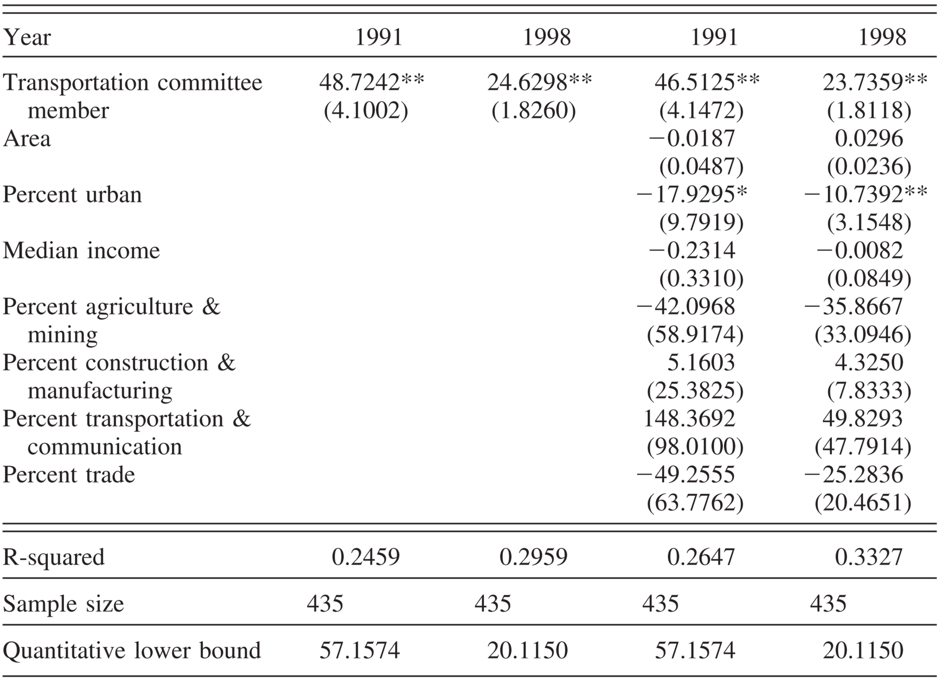
Source: Table 2 of Knight (2005)

Are you convinced?

Alternative explanation of OLS results

Legislators may join the committee

because their districts need more highways

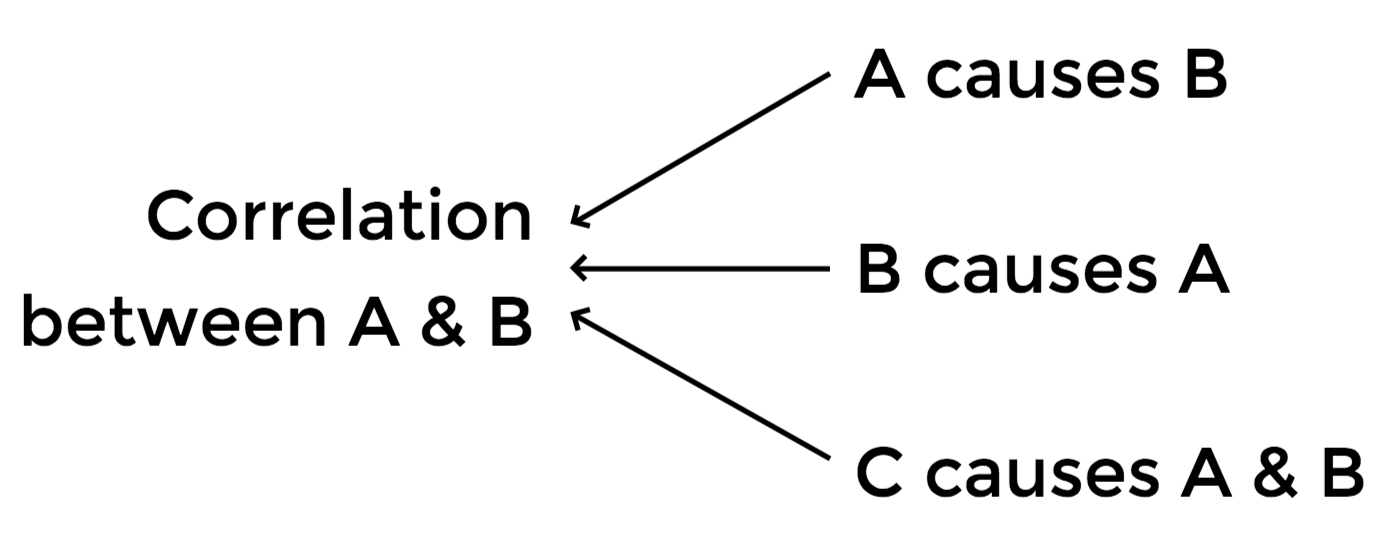
In need of highways

Alternative empirical specification #1

Restrict the sample to those districts that can be matched

g_{dt}=\mu_d+\beta P_{dt}+\mathbf{X}_{dt}\mathbf{\Gamma}+\varepsilon_{dt}

g_{dt}=\mu_d+\beta P_{dt}+\mathbf{X}_{dt}\mathbf{\Gamma}+\varepsilon_{dt}

District fixed effects

Control for unobservable time-invariant district characteristics

But due to the redrawing of districts in 1992,

some districts cannot be matched between 1991 and 1998

Aggregate at the state level by taking the averages

\bar{g}_{st}=\mu_s+\beta \bar{P}_{st}+\mathbf{\bar{X}}_{st}\mathbf{\Gamma}+\varepsilon_{st}

\bar{g}_{st}=\mu_s+\beta \bar{P}_{st}+\mathbf{\bar{X}}_{st}\mathbf{\Gamma}+\varepsilon_{st}

State fixed effects

Fixed effects estimation results

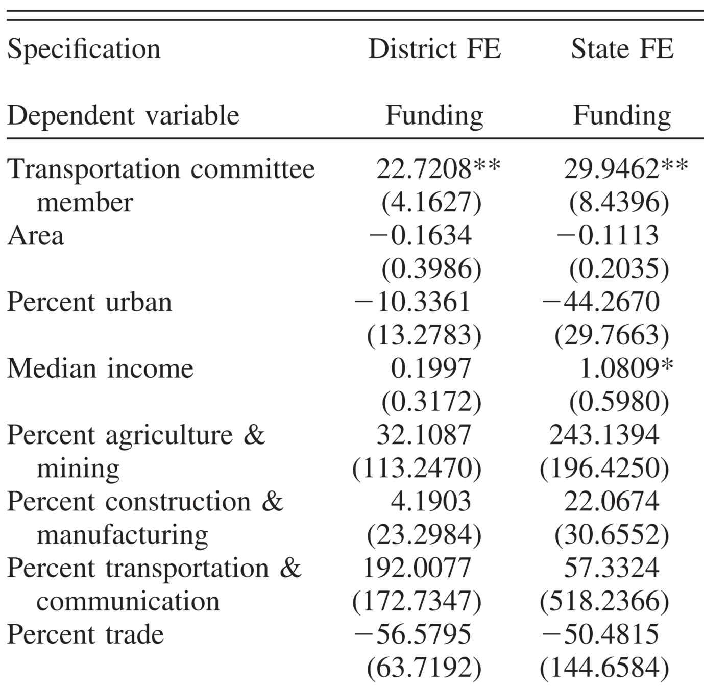
Source: Table 5 of Knight (2005)

Are you convinced?

Alternative explanation of FE results

Committee members in 1991 leave the committee

because their districts no longer need more highways

Decline in the need of highways

Alternative empirical specification #2

Newly elected legislators are more likely to join the committee

Use the indicator of being newly elected as an instrument

Are you convinced?

First-stage does work: 8.5 pt increase (sample mean 15%)

Threats to the exclusion restriction

Newly elected legislators are less powerful

This may directly affect the allocation of funds to their district

Takeaway

The positive correlation

between committee membership & allocated funds

Consistent with theoretical predictions

from legislative bargaining model

Application:

Presidentialism

vs

Parliamentarism

Adapted from Persson et al. (2000 JPE)

(See also sections 10.2-10.3 of Persson and Tabellini 2000)

Motivation:

Impacts of political institutions

on economic policies

We have seen the impacts of

Electoral rules (Lecture 3)

Term limits (Lecture 4)

Another major difference in political institutions across countries

Presidentialism vs Parliamentarism

A Model of

Fiscal Policy-making

Players

Three legislators, $J \in \{1,2,3\}$

Each represents a region (or a group of voters)

Without loss of generality, assume:

Legislator 1 is in charge of proposing the tax policy

Legislator 2 is in charge of proposing the expenditure policy

Legislator 3 is the minority party member

Preference

Legislator $J$'s payoff

y-\tau+H(g)+f^J

y-\tau+H(g)+f^J

Exogenous income

y

\tau

\tau

Lump-sum tax

g

Public goods (benefiting all legislators)

f^J

f^J

Transfer to region $J$

Preference

Legislator $J$'s payoff

y-\tau+H(g)+f^J

y-\tau+H(g)+f^J

Each legislator can be thought of as

a citizen-candidate who won the election in each region

Actions

Legislator 1 proposes $\tau$

Legislator 2 proposes $g$, $\{f^J\}$

e.g. Finance Minister

Member of Congress Committee on Taxation

e.g. Other Ministers

Members of Congress Committees on Expenditure

All legislators vote on these proposals

Actions

Legislator 1 proposes $\tau$

Legislator 2 proposes $g$, $\{f^J\}$

All legislators vote on these proposals

Which action follows which

depend on the form of government

Modelling

forms of government

Differences between

Presidentialism and Parliamentarism

Major difference: how the chief executive is elected

Other important differences: How legislature makes policies

But we do not model this here

Presidentialism

Different congressional committees hold proposal power over different policy issues

Separation of Power

=

Taxation

Spending

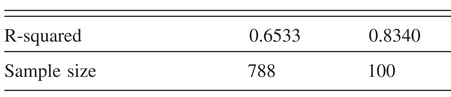
Parliamentarism

Ruling party legislators propose almost all bills

A disagreement within ruling party members leads to a government crisis (vote of no confidence 「内閣不信任決議」)

June 1993: Vote of no confidence against Prime Minister Miyazawa was approved as some LDP members voted in favour

Image source: www.huffingtonpost.jp/2014/11/20/general-election_n_6190126.html

Legislative cohesion

=

Fiscal policy in

presidentialism

Timing of Events in Presidentialism

Legislator 1 proposes total tax revenue, $\tau$

Legislators vote on the tax proposal

If rejected, the default policy, $g=f^1=f^2=f^3=0$, is implemented

Legislator 2 proposes expenditures on public goods ($g$) and transfer to each region ($f^1, f^2, f^3$)

Legislators vote on the expenditure proposal

If rejected, the default policy, $\bar{\tau}=0$, is implemented

Backward induction

Legislator 1 proposes total tax revenue, $\tau$

Legislators vote on the tax proposal

If rejected, the default policy, $g=f^1=f^2=f^3=0$, is implemented

Legislator 2 proposes expenditures on public goods ($g$) and transfer to each region ($f^1, f^2, f^3$)

Legislators vote on the expenditure proposal

If rejected, the default policy, $\bar{\tau}=0$, is implemented

Legislators 1 & 3's optimal voting

on the expenditure proposal

Both prefer anything only slightly better than the default policy

Legislator $J$ accept the proposal if

g \geq 0, f^J \geq 0

g \geq 0, f^J \geq 0

(Assuming they will accept when indifferent between the bill and the default policy)

Backward induction

Legislator 1 proposes total tax revenue, $\tau$

Legislators vote on the tax proposal

If rejected, the default policy, $g=f^1=f^2=f^3=0$, is implemented

Legislator 2 proposes expenditures on public goods ($g$) and transfer to each region ($f^1, f^2, f^3$)

Legislators vote on the expenditure proposal

If rejected, the default policy, $\bar{\tau}=0$, is implemented

Legislator 2's optimal proposal on expenditure

Choose policies to solve

\max_{g, \{f^J\}} y-\tau+H(g)+f^2

\max_{g, \{f^J\}} y-\tau+H(g)+f^2

subject to

3\tau=g+\sum_Jf^J

3\tau=g+\sum_Jf^J

g \geq 0, f^1\geq 0, f^3\geq 0

g \geq 0, f^1\geq 0, f^3\geq 0

First, there is no need to provide positive $f^1, f^3$ to pass the bill

\max_g y-\tau+H(g)+(3\tau-g)

\max_g y-\tau+H(g)+(3\tau-g)

Legislator 2's optimal proposal on expenditure

First order condition:

H_g(g^{PR})=1

H_g(g^{PR})=1

The remaining tax revenue is used for transfer to region 2

f^{2,PR}=3\tau-g^{PR}

f^{2,PR}=3\tau-g^{PR}

f^{1,PR}=0

f^{1,PR}=0

f^{3,PR}=0

f^{3,PR}=0

Backward induction

Legislator 1 proposes total tax revenue, $\tau$

Legislators vote on the tax proposal

If rejected, the default policy, $g=f^1=f^2=f^3=0$, is implemented

Legislator 2 proposes expenditures on public goods ($g$) and transfer to each region ($f^1, f^2, f^3$)

Legislators vote on the expenditure proposal

If rejected, the default policy, $\bar{\tau}=0$, is implemented

Legislator 1's optimal tax proposal

Choose $\tau$ to solve

\max_{\tau} y-\tau+H(g^{PR})+f^{1,PR}

\max_{\tau} y-\tau+H(g^{PR})+f^{1,PR}

subject to

3\tau=g^{PR}+f^{2,PR}

3\tau=g^{PR}+f^{2,PR}

f^{1,PR}=0

f^{1,PR}=0

H_g(g^{PR})=1

H_g(g^{PR})=1

Starting with $\tau=0$, legislator 2 will first spend any increase in $\tau$ on $g$

Legislator 1's optimal tax proposal

Starting with $\tau=0$, legislator 2 will first spend any increase in $\tau$ on $g$

Until the marginal utility from $g$ reaches 1

Then legislator 2 will spend any extra increase in $\tau$ on $f^2$

Legislator 1 benefits as well

Legislator 1 no longer benefits

So it's optimal for legislator 1 to set

\tau^{PR} = g^{PR}

\tau^{PR} = g^{PR}

Both legislators are happy to accept

Fiscal policy in

parliamentarism

Timing of Events in Parliamentarism

Legislators 1 & 2 (i.e. the cabinet) jointly propose the policy package, $\tau, g, f^1, f^2, f^3$

Legislators vote on the proposal

If rejected, the cabinet resigns; the default policy, $\bar{\tau}=g=f^1=f^2=f^3=0$, is implemented

Transfer to opposition's region

No support from the opposition is needed to pass the bill

f^3=0

f^3=0

Public goods & transfer to ruling party's regions

Legislators 1 & 2 jointly maximize their payoffs

Given $\tau$, they choose $g$ to solve

\max_{g, \{f^J\}} 2[y-\tau+H(g)]+f^1+f^2

\max_{g, \{f^J\}} 2[y-\tau+H(g)]+f^1+f^2

=\max_g2[y-\tau+H(g)]+3\tau-g

=\max_g2[y-\tau+H(g)]+3\tau-g

Govt budget constraint & $f^3=0$

FOC w.r.t. $g$

2H_g(g)=1

2H_g(g)=1

Size of government

Legislators 1 & 2 jointly maximize their payoffs

Given the optimal $g^{PA}$, they choose $\tau$ to solve

\max_{\tau\in[0,y]} 2[y-\tau+H(g^{PA})]+3\tau-g^{PA}

\max_{\tau\in[0,y]} 2[y-\tau+H(g^{PA})]+3\tau-g^{PA}

FOC w.r.t. $\tau$

1>0

1>0

Extracting income from region 3

to split it among the two regions

\tau^{PA}=y

\tau^{PA}=y

Comparative politics

Presidentialism

Parliamentarism

H_g(g^{PR})=1

H_g(g^{PR})=1

2H_g(g^{PA})=1

2H_g(g^{PA})=1

g^{PR} < g^{PA}

g^{PR} < g^{PA}

Public good provision

Regional transfer

f^1=f^2=f^3=0

f^1=f^2=f^3=0

f^1+f^2=y-g^{PA}

f^1+f^2=y-g^{PA}

f^3=0

f^3=0

Tax revenue

\tau = g^{PR}

\tau = g^{PR}

\tau = y

\tau = y

<

Evidence on the impact of forms of government

Persson and Tabellini (2004 AER)

Causal evidence?

Hard to prove causality running from forms of govt to policies

Forms of government rarely change

Thus impossible to separate their impact

from that of country characteristics

Causal evidence?

We can only check

if correlation is consistent with the theoretical prediction

Persson and Tabellini (2004)

Run cross-country regressions of fiscal policies on forms of govt

y_i = \beta S_i+\mathbf{Z}_i\mathbf{\Gamma}+\varepsilon_i

y_i = \beta S_i+\mathbf{Z}_i\mathbf{\Gamma}+\varepsilon_i

S_i

S_i

Indicator of presidentialism in country $i$

Theory predicts $\beta < 0$ when $y_i$ is the size of government

Persson and Tabellini (2004)

Run cross-country regressions of fiscal policies on forms of govt

y_i = \beta S_i+\mathbf{Z}_i\mathbf{\Gamma}+\varepsilon_i

y_i = \beta S_i+\mathbf{Z}_i\mathbf{\Gamma}+\varepsilon_i

\mathbf{Z}_i

\mathbf{Z}_i

Per capita GDP

Trade openness

Population

% of those aged 16-54

% of those aged over 65

Years of being democracy

Quality of democracy (Freedom House Index)

Dummy for majoritarian elections

(cf. Lecture 3)

Dummy for federal states

Dummy for OECD countries

Dummies for continents

Dummies for legal origins

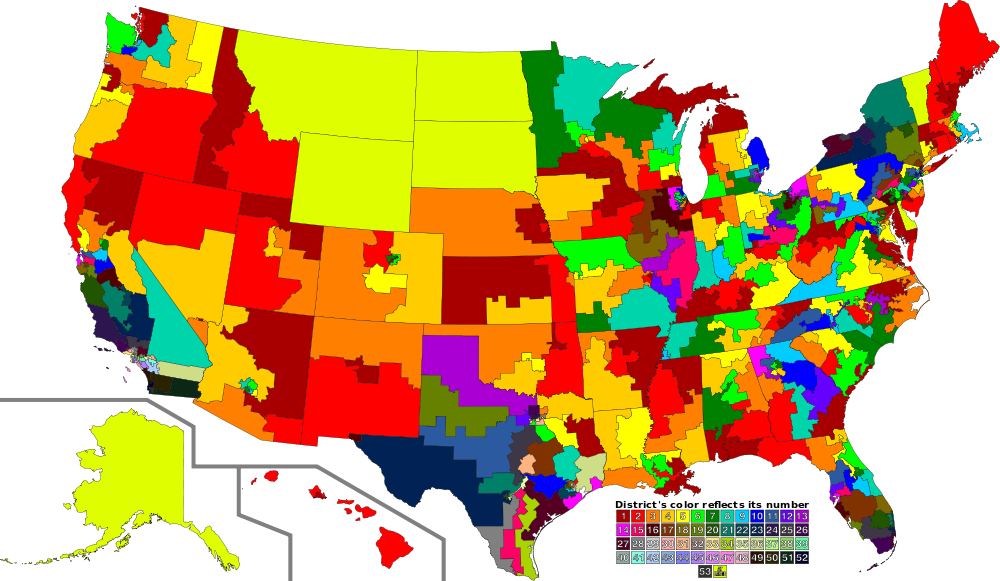
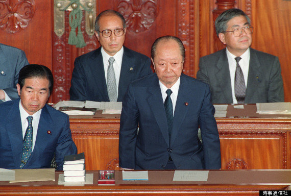
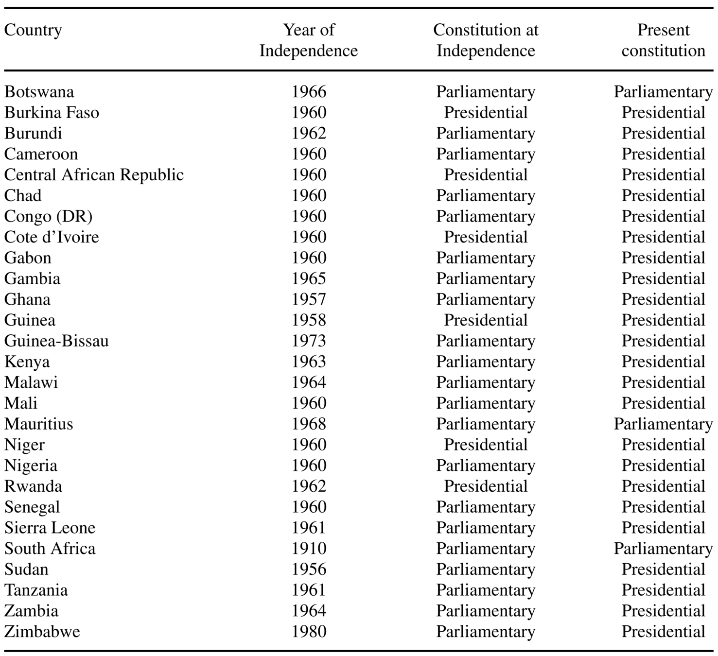
Forms of government across the world in 1998

Source: Figure 4.1 of Persson and Tabellini (2003)

Presidential

Parliamentary

Not democratic

(S_i=1)

(S_i=1)

(S_i=0)

(S_i=0)

(excluded from the sample)

Unconditional mean comparison

Fiscal policy (as % of GDP)	Central govt expenditure	Social protection
Presidential system	22.2% (7.2)	4.8% (4.6)
Parliamentary system	33.3% (10.0)	9.9% (7.0)
p-value for two-sample t-test

Source: Table 1 of Persson and Tabellini (2004)

Note: Standard deviation in parentheses

0.00

OLS estimation results

Dep. Var. (as % of GDP)	Central govt expenditure	Central govt revenue	Government deficit	Social protection
Presidentialism	-5.18*** (1.93)	-5.00** (2.47)	0.16 (1.15)	-2.24* (1.11)
# observations	80	76	72	69