Models of Lobbying
Lecture 7, Political Economics I
OSIPP, Osaka University
1 December, 2017
Masa Kudamatsu
Motivation
We have seen
how elections and legislative bargaining affect the choice of policies
But policy-making also depends on lobbying by interest groups
e.g. NRA (National Rifle Association) in U.S.

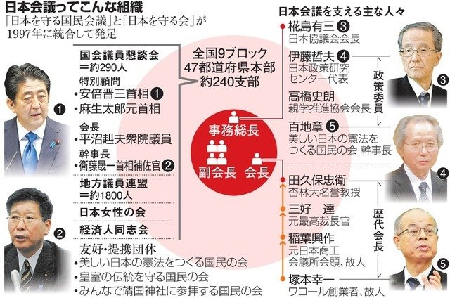
e.g. 日本会議
But policy-making also depends on lobbying by interest groups
Motivation (cont.)
Motivation (cont.)
In what way
do these interest groups
influence policy-making?
The literature (and this lecture)
almost exclusively focuses on lobbying in U.S.
Partly because good data is available
Lobbying in other countries (including Japan)
is completely an open question
Models of lobbying
There is no widely accepted model to analyze lobbying
Contest Model
(How lobbyists affect policy is blackboxed)
Existing models can be categorised as below
Quid Pro Quo
Models
Offering money to policy-makers contingent on enacted policy
Informational Lobbying
Models
Providing information on which policy benefits policy-makers
Quid Pro Quo Models
Quid Pro Quo models
Popular in the 1990s
Several variants, but they all assume
Interest groups promise to pay "bribes" to politicians
if their preferred policy is chosen
They can commit to this promise once the policy is chosen
Or politicians can commit to the policy after receiving bribes in advance
Most popular was the common agency model
Common Agency Model
also known as the menu auction model
Originally proposed by Bernheim and Whinston (1986)
as a version of the principal-agent model
with many principals and one agent
Grossman and Helpman (1994) apply this model to trade policy-making process influenced by interest groups
We follow a version used
by Section 7.3 of Persson and Tabellini (2000)
Model in a nutshell
1
Each interest group \(J\) simultaneously propose
a contribution schedule \(C^J(\mathbf{g})\), to maximize
\(\mathbf{g}\): Vector of policies
\(C^J(\mathbf{g})\): the amount of \(J\)'s contribution
if the policy-maker implements \(\mathbf{g}\)
We assume interest groups can commit to their contribution schedule proposal
W^J(\mathbf{g}) - C^J(\mathbf{g})
\(W^J(\mathbf{g})\): \(J\)'s payoff from policies
2
Model in a nutshell
Observing \(C^J(\mathbf{g})\), the single policy-maker sets \(\mathbf{g}\) to maximize
\eta V(\mathbf{g}) + (1-\eta) \sum_J C^J(\mathbf{g})
\(V(\mathbf{g})\): the policy-maker's payoff from policies
Social welfare, if the policy-maker is benevolent
e.g.
Weighted sum of citizen payoffs, if the election is modeled as in the probabilistic voting model
How much the policy-maker can be corrupt
\(\eta \in [0,1]\): Weight on the policy-maker's own preference
e.g.
Degree of benevolence, if \(V(\mathbf{g})\) is social welfare
Equilibrium
Interest group \(J\)'s optimal contribution schedule is given by
with some \(B_J>0\)
C^{J*}(\mathbf{g}) = \max\{W^J(\mathbf{g}) - B_J, 0\}
Consequently, the policy-maker maximizes
\eta V(\mathbf{g}) + (1-\eta) \sum_J W^J(\mathbf{g})
that is, the weighted sum of payoffs with interest groups' weight being \(1-\eta\)
Applications
Trade policies (Grossman and Helpman 1994 AER)
Evidence: Goldberg and Maggi (1999 AER) and Gawande and Bandyopadhyay (2000 Restat) for U.S.
Mitra et al. (2002 Restat) for developing countries
Theoretical extensions
Citizen-candidate model (Besley and Coate 2001 Restud)
Legislative-bargaining model (Helpman and Persson 2001)
Endogenous lobby formation (Mitra 1999 AER)
Other quid pro quo models of lobbying
Legislative vote buying model of Groseclose and Snyder (1996)
Bribery contingent on voting, not the enacted policy
Applied by Diermeier and Myerson (1999 AER) to endogenize legislative committees' agenda-setting power
The poor citizens may prefer dismantling checks & balances
(i.e. legislature can veto president's policy-making)
if the rich bribes the president
Evidence against quid pro quo models of lobbying
Measuring money given by interest groups
Organizations wishing to give contributions to federal candidates
must create PACs (political action committees)
PACs must raise voluntary donations from individuals
Corporate PAC contributions: corporate managers
Labor PAC contributions: labor union members
In 2000, about 3000 PACs contributed to federal candidates
1,400 associated with corporations
240 associated with labor unions
Panel regression
y_{it} =\alpha C_{it}+\beta L_{it}+\mu_i+\eta_t+\varepsilon_{it}
% of times legislator \(i\) votes in line with Chamber of Commerce during Congress period \(t\)
y_{it}
C_{it}
Amount of contributions from corporate PACs
received by legislator \(i\) during Congress period \(t\)
L_{it}
Amount of contributions from labor PACs
received by legislator \(i\) during Congress period \(t\)
If contributions are effective, we should see
\alpha>0, \beta<0
Results
| FE estimates | Mean [s.d.] | |
|---|---|---|
| Corporate Contributions |
0.02 | 6.53 [5.99] |
| Labor Contributions |
-0.13 | 4.48 [5.39] |
| # of observations | 3400 |
Both estimates are not significantly different from zero
Dependent variable: % of times voting for Chamber of Commerce
1 s.d. increase in contributions raise the voting score only by
0.12 ppt (corporate) / -0.70 ppt (labor)
Source: Table 2 of Ansolabehere et al. (2003)
(Standard errors are not reported in the paper...)
Taking stock
Although it's not causal, available evidence is inconsistent with the quid pro quo models' assumption that politicians receive money in return for their policy choice
Contest Model
We follow a version used by Kang (2016 Restud)
Motivation
Campaign contributions are not the only way for the interest group to interact with politicians
Interest groups can hire lobbyists to contact with politicians
Money involved
in U.S. in 2012
Campaign contributions
Interest
Groups
Politicians
Lobbyists
Hire
?
$750,000,000
$3,500,000,000
Source: de Figueiredo and Richter (2014), p. 165
Question
Do lobbying expenditures influence politicians' choice of policies?
Kang (2016 Restud) attempts to answer this question
by structurally estimating the contest model
Measuring the enactment of a policy
Collect all the bills on the energy sector
introduced during the 110th Congress
(2007-2008: last 2 years of George W Bush's 2nd-term presidency)
Including those the committees didn't submit to the floor
Divide a bill into sections
One bill may deal with several policies
A bill section deals with one specific policy
Measuring the enactment of a policy (cont.)
Obtain word frequencies of each bill section

Image source: khorn2.onmason.com/author/khorn2/
Measuring the enactment of a policy (cont.)
Treating word frequencies as a vector,
measure the angle between a pair of bill sections
Image source: www.mathsisfun.com/algebra/vectors-dot-product.html
Measuring the enactment of a policy (cont.)
\cos \theta = 1
if relative frequencies of all words are the same
\cos \theta = 0
if no single word is used in common
Treat bill sections as the same policy if
\cos\theta \geq 0.985

Then look at the status of the last bill
among all bill sections dealing with one policy
Measuring the enactment of a policy (cont.)
Bills are typically amended throughout Congress session
| Status | # of policies | % of policies |
|---|---|---|
| Enacted | 45 | 8.4% |
| Reported | 106 | 19.7% |
| Not reported | 387 | 71.9% |
Source: Table 1 of Kang (2016)
Data on the U.S. lobbying industry
Lobbying Disclosure Act of 1995
requires all lobbying firms to report (twice a year):
Client names
Revenue received from each client
List of bills they lobby for/against (for each client)
Names of individual lobbyists involved for each client
Data can be downloaded at Senate Office of Public Records (SOPR)
Center for Responsive Politics summarises the data
Measuring lobbying expenditure
The lobbying industry data identify
559 firms and trade associations in the energy sector
Total lobbying expenditure: $607.9m
Median lobbying expenditure: $0.16m
Top 10% accounts for 76% of total expenditure
Source: Kang (2016), page 273
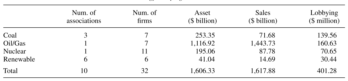
Measuring lobbying expenditure (cont.)
Source: Table 2 of Kang (2016)
Group these lobbying firms and trade associations
into four sub-sectors
Coal
Oil/Natural Gas
Nuclear
Renewable energy
Measuring which policy was lobbied
Assume a coalition lobbies for/against all policies within a bill mentioned in the dataset
% of policies each lobbying coalition participates in lobbying
| Coal | 50% |
| Oil / Natural Gas | 67% |
| Nuclear | 49% |
| Renewable | 62% |
Source: Table 3 of Kang (2016)
Data limitation & Case for structural estimation
Each coalition's lobbying expenditure is observed only in total
Use the equilibrium condition to allocate into different policies
No counterfactual to estimate the impact of lobbying expenditure
Use the model to estimate the probability of policy adoption in the absence of lobbying
Model: Players and Preference
Lobbyists of two types
Those in favor of the policy, \(l \in L_f\)
Those against the policy, \(l \in L_a\)
derive a payoff of \(v_l > 0\) if policy is adopted
derive a payoff of \(v_l < 0\) if policy is adopted
Model: Timing of Events
1
2
3
Each lobbyist simultaneously decides whether to lobby
by incurring the entry cost, \(c\)
Observing all the other lobbyists' decision on participation, each lobbyist \(l\) decides how much to spend \(s_l\)
The policy is adopted with probability
p(\mathbf{s}_f, \mathbf{s}_a, \pi)\equiv \frac{\pi + \beta_f \sum_{i \in L_f} (s_i)^\gamma}{1+\beta_f \sum_{i \in L_f} (s_i)^\gamma+\beta_a\sum_{j \in L_a} (s_j)^\gamma}
Notice this is a version of the contest success function that we saw in Lecture 6a
Model: Policy adoption probability
p(\mathbf{s}_f, \mathbf{s}_a, \pi)\equiv \frac{\pi + \beta_f \sum_{i \in L_f} (s_i)^\gamma}{1+\beta_f \sum_{i \in L_f} (s_i)^\gamma+\beta_a\sum_{j \in L_a} (s_j)^\gamma}
\(\pi\) if no one lobbies
Reflecting legislators' preference, institutional features, etc.
Policy adoption probability (cont.)
p(\mathbf{s}_f, \mathbf{s}_a, \pi)\equiv \frac{\pi + \beta_f \sum_{i \in L_f} (s_i)^\gamma}{1+\beta_f \sum_{i \in L_f} (s_i)^\gamma+\beta_a\sum_{j \in L_a} (s_j)^\gamma}
Not one even if only those in favor lobby (i.e. \(s_l=0\) for all \(l \in L_a\))
Consistent with the lobbying expenditure data for U.S.
Not zero
against
for all \(l \in L_f\)
Policy adoption probability (cont.)
p(\mathbf{s}_f, \mathbf{s}_a, \pi)\equiv \frac{\pi + \beta_f \sum_{i \in L_f} (s_i)^\gamma}{1+\beta_f \sum_{i \in L_f} (s_i)^\gamma+\beta_a\sum_{j \in L_a} (s_j)^\gamma}
We assume \(\gamma < 1\)
Consistent with the lobbying expenditure data for U.S.
Implies a larger # of participating lobbyists is more effective, holding the total amount of expenditure constant
This ensures multiple participating lobbyists in the equilibrium
Equilibrium
The lobbying expenditure game has the unique Nash equilibrium
See Appendix B of Kang (2016) for proof
The lobbying participation game has multiple equilibria
Assume that the equilibrium with the highest sum of payoffs of all players is selected
Structural estimation
Pick the parameters of the model (\(\beta_f, \beta_a, \gamma\), etc.)
to maximize the likelihood of observing
Whether each lobbyist participates for
Total expenditure by each lobbyist over all policies
Whether each policy is adopted
Findings
\hat{p}(\hat{\mathbf{s}_f}, \hat{\mathbf{s}_a}, \hat{\pi}) -
\hat{\pi} = 0.00054
95% confidence interval: [0.00021, 0.00415]
Impact of lobbying on policy adoption rate
Average return to lobbying expenditure
\frac{[\hat{p}(\hat{s}_l, \hat{\mathbf{s}}_{-l}, \hat{\pi}) - \hat{p}(0,\tilde{\mathbf{s}}_{-l},\hat{\pi})]
\hat{v_l}}{\hat{s_l}} -\hat{s_l} \in [1.37,1.52]
\(\tilde{\mathbf{s}}_{-l}\) is the other lobbyist expenditure as the equilibrium response to \(s_l=0\)
For coal coalition: \(v_l\) is $802 million; \(s_l\) is $291,588
Taking stock
Probability of policy adoption changes very little due to lobbying
But return to lobbying exceeds 100%
because of a very high gain from policy adoption
How lobbyists affect policy-making, however, is blackboxed
Informational lobbying models
Motivations
One role of lobbyists is believed to be
the provision of information to politicians
Politicians do not know what policies benefit citizens the most (and themselves through their re-election probability)
Interest groups have such information
They may want to lobby themselves or hire lobbyists
to convey such information to politicians
Models of informational lobbying
Can be categorized into two groups
1
2
Cheap talk
Costly or verifiable information
Lobbying with verifiable information
Model
Players: Policy-maker \(L\) and two interest groups \(j \in{A,B}\)
Policy: \(D \in \{a, b\} \)
Preference over policy:
Policy-maker \(L\): \(V_L\) if \(D=s\); 0 otherwise
Group \(A\): \(W_A\) if \(D=a\); 0 otherwise
Group \(B\): \(W_B\) if \(D=b\); 0 otherwise
State of the world: \(s \in \{a, b\} \)
i.e. Which policy benefits citizens more
Prior: \(\Pr(s=a) = p < 1/2 \)
Model: Signal on the state of the world
Interest groups can invest \(C_j\)
to acquire the signal, \(\sigma\), on the state of the world
\Pr(s=a|\sigma=a)=\Pr(s=b|\sigma=b)=q\in(\frac{1}{2},1)
i.e. the signal is informative (q>1/2) but not fully accurate (q<1)
Timing of events
Groups \(A\) and \(B\) simultaneously decide whether to acquire signal on the state of the world, \(\sigma\in\{a,b\}\), at the cost of \(C_j\)
1
Policy-maker \(L\) observes the decisions by \(A\) and \(B\), but not the acquired information, \(\sigma\)
2
Groups \(A\) and \(B\) simultaneously decide whether to send a message \(m_j\in\{a,b\}\) to \(L\)
3
Observing messages \(m_a\) and \(m_b\), \(L\) decides whether to learn the state of the world on his/her own at the cost of \(c\)
4
\(L\) decides which policy to implement, \(a\) or \(b\)
Group \(j\) gets punished by fine \(f\) if \(m_j \neq s\)
Results
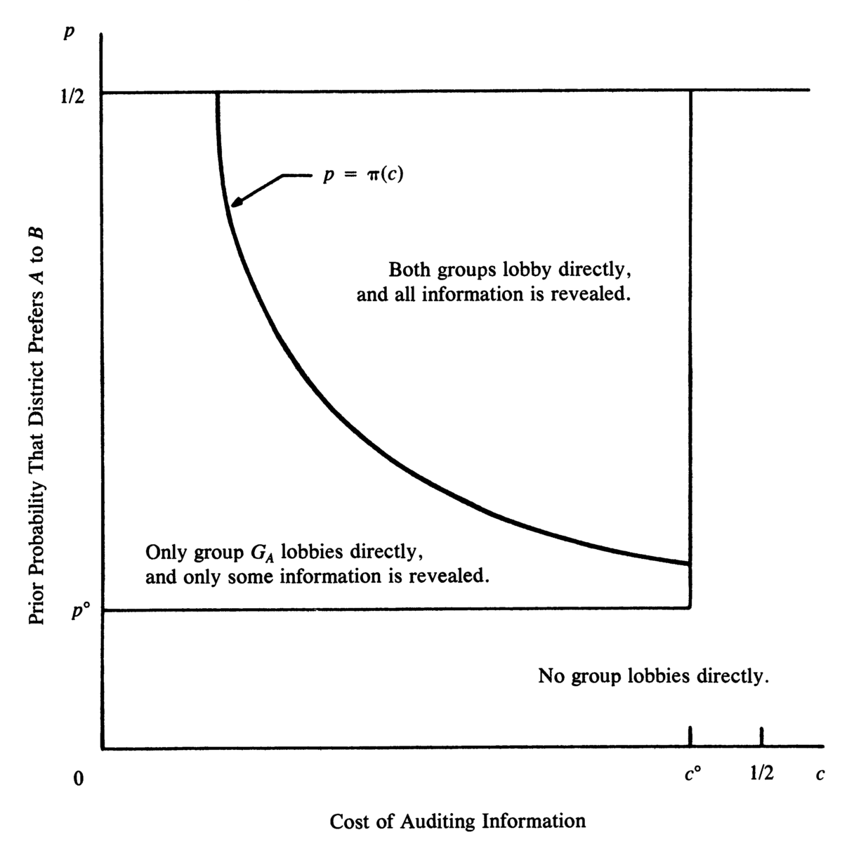
Source: Figure 1 of Austin-Smith and Wright (1994)
Application
Propose a similar model of informational lobbying
(which incorporates the legislative bargaining model)
to explain why
lobbying activities are less prevalent in parliamentary democracies
Cheap Talk
We follow a simpler exposition
by Chapter 4 of Grossman and Helpman (2001)
Model
One-dimensional policy \(p\)
Which policy is desirable for the policy-maker depends on the state of the world, \(\theta\), observed only by interest group(s)
Policy-maker's payoff:
-(p-\theta)^2
i.e. The value of \(\theta\) is the best policy
Interest group's payoff:
-(p-\theta-\delta)^2
\(\delta > 0\) is the bias in the group's policy preference
Players: Policy-maker and Interest group
Timing of Events
1
2
3
4
Nature picks the value of \(\theta\) according to its distribution \(F(\theta)\)
Interest group sends a message \(\sigma\)
Interest group observes \(\theta\), but policy-maker doesn't
Which may or may not be the same as \(\theta\)
Policy-maker updates their belief on \(\theta\), denoted by \(\tilde{\theta}\)
by observing the message \(\sigma\)
5
Policy-maker chooses the policy \(p\)
Equilibria
In cheap talk games,
there are multiple Perfect Bayesian Nash equilibria
One of such is that policy-maker does not believe the message is true (known as the "babbling equilibrium")
See Chapter 18 of Tadelis (2013) for detail
But if the bias \(\delta\) is small enough,
there exists an equilibrium where interest groups report the true \(\theta\) and the policy-maker believes it
We illustrate this with a simple two state case
If there are two states of the world
Suppose \(\theta \in \{\theta_L, \theta_H\} \), with \( \theta_H>\theta_L \)
When does the interest group has no incentive to lie?
Suppose the policy-maker believes the interest group's message
When \(\theta=\theta_H\)
telling a lie
telling
the truth
-\delta^2 > -(\theta_L-\theta_H-\delta)^2
If there are two states of the world
Suppose \(\theta \in \{\theta_L, \theta_H\} \), with \( \theta_H>\theta_L \)
When does interest group has no incentive to lie?
Suppose the policy-maker believes the interest group's message
When \(\theta=\theta_L\)
telling a lie
telling
the truth
-\delta^2 \gtrless -(\theta_H-\theta_L-\delta)^2
Tell the truth if
\delta \leq \frac{\theta_H-\theta_L}{2}
With continuous states of the world
The condition for not telling \(\theta_1\) when \(\theta=\theta_2 \)
\delta \leq \frac{\theta_2-\theta_1}{2}
Consider a pair of two values of \(\theta\), (\(\theta_1, \theta_2) \) with \(\theta_1 < \theta_2\)
does not hold for all pairs of \(\theta\)
Full information revelation cannot be an equilibrium
With continuous states of the world
Instead, a message like
\(\theta\) is in the range between \(\theta_L\) and \(\theta_H\)
can be an equilibrium if \(\delta\) is sufficiently small
If we suppose the uniform distribution of \(\theta\)
Then policy-maker chooses policy \(\frac{\theta_L+\theta_H}{2}\)
(i.e. the expected value of \(\theta\) given the message)
See Section 4.1.4 of Grossman and Helpman (2001)
With two interest groups of opposite bias
Krishna and Morgan (2001) extend the cheap talk model
by adding one more message sender (i.e. two interest groups)
Denote each group's bias by \(\delta_1, \delta_2\)
Then if \(\delta_1 < 0 < \delta_2\) (i.e. two interest groups have opposite bias)
the policy-maker may learn more by listening to both,
instead of listening to only one of them
With two interest groups of opposite bias (cont.)
\theta
Group 1 sends a message whether \(\theta \leq \bar{\theta}_1\)
\bar{\theta}_1
Group 2 then sends a message whether \(\theta \leq \bar{\theta}_2 (< \bar{\theta}_1)\)
\theta
\bar{\theta}_2
Policy-maker, updating the belief, sets the policy
\theta
\frac{\theta_{min}+\bar{\theta}_2}{2}
\frac{\bar{\theta}_2+\bar{\theta}_1}{2}
\frac{\bar{\theta}_1+\theta_{max}}{2}
With two interest groups of opposite bias (cont.)
(2) Group 2 is indifferent between policies
\bar{\theta}_2
\theta
\frac{\theta_{min}+\bar{\theta}_2}{2}
\frac{\bar{\theta}_2+\bar{\theta}_1}{2}
\frac{\bar{\theta}_1+\theta_{max}}{2}
For this to be an equilibrium:
(1) Group 1 is indifferent between policies
\frac{\bar{\theta}_2+\bar{\theta}_1}{2}
&
when \(\theta = \bar{\theta}_1\)
\frac{\theta_{min}+\bar{\theta}_2}{2}
&
\frac{\bar{\theta}_2+\bar{\theta}_1}{2}
\bar{\theta}_1
\frac{\bar{\theta}_1+\theta_{max}}{2}
when \(\theta = \bar{\theta}_2\)
Such a pair of \(\bar{\theta}_1, \bar{\theta}_2 \) can exist when \(\delta_1<0<\delta_2\)
Evidence on informational lobbying
Data on the U.S. lobbying industry
Lobbying Disclosure Act of 1995
requires all lobbying firms to report (twice a year):
Client names
Revenue received from each client
List of bills they lobby for/against (for each client)
Names of individual lobbyists involved for each client
Data can be downloaded at Senate Office of Public Records (SOPR)
Center for Responsive Politics summarises the data
Data on the U.S. lobbying industry (cont.)
Collection of biographies of lobbyists
compiled by Columbia Books and Information Services
Of which about 17,000 can be matched in www.lobbyists.info
About 37,000 lobbyists for 1999-2008 in the SOPR data
Source: Bertrand et al. (2014), p. 3889
Measuring lobbyists' expertise
From the SOPR data:
Obtain revenues a lobbyist earns from each policy issue
(see next slide for how)
1/4 of lobbyists are specialists, defined this way
Those with political experiences are less likely to be specialists
Define a specialist lobbyist as the one whose revenue from one policy issue exceeds 25% of his/her total revenue
Source: Bertrand et al. (2014), pp. 3897-3900
Measuring each lobbyist's expertise (cont.)
(lobbyist 's revenue from policy issue ) is obtained by
V_{il}
V_{il}=\sum_t \sum_r V_{ilrt}
where VilrtV_{ilrt}Vilrt is the revenue for lobbyist lll for issue iii
from client rrr in year ttt, which in turn given by
V_{ilrt}=\frac{V_{rt}}{I_{rt}L_{rt}}
VrtV_{rt}Vrt Lobbying firm revenue from client rrr in year ttt
IrtI_{rt}Irt # of issues the lobbying firm worked for client rrr in year ttt
LrtL_{rt}Lrt # of lobbyists working for client rrr in year ttt
(All obtained from the SOPR dataset)
Measuring lobbyists connected to politicians
For each lobbyist in the SOPR data
obtain his/her campaign contributions to any politician
from the Federal Election Commission data
If a lobbyist makes one contribution to a politician
define this lobbyist as connected to the politician
Empirical specification
S_{ptj} =\delta_1+\delta_21(j=1)+\gamma_p+\delta_t+\eta_{ptj}
\(S_{ptj}\): Share of opposite party lobbyists of type \(j\) connected to politician \(p\) for congress period \(t\)
\(j\): Indicator of lobbyists being specialist
If lobbyists provide information to politicians, we should see
\delta_2>0
This cannot be explained by quid pro quo models of lobbying
Results
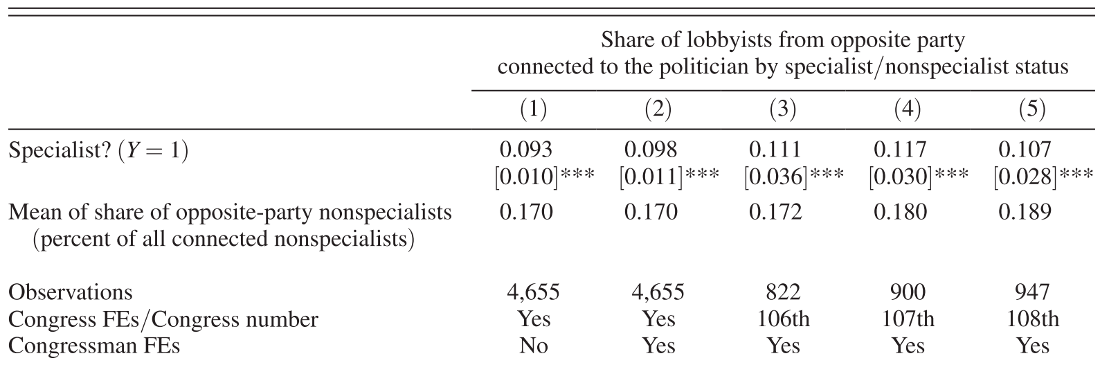
Source: Table 7 of Bertrand et al. (2014)
% of opposite party lobbyists
17%
among non-specialists
27%
among specialists
vs
Note: Standard errors clustered at the politican level are reported in brackets
Results
Source: Table 7 of Bertrand et al. (2014)
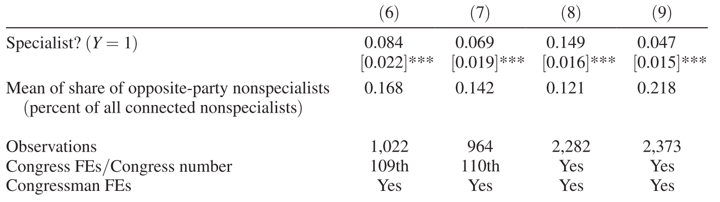
Democrat
politicians
Republican
politicians
Not driven by particular congress periods
Not driven by either of the parties
Note: Standard errors clustered at the politican level are reported in brackets
Summary
Lesson #1
The quid pro quo view of lobbying seems unlikely
Politicians do not appear to respond to contributions
in their policy choice
Lesson #2
Lobbying affects the probability of policy adoption only a little
But the value of a policy is so big that the return from lobbying expenditure exceeds 100%
Lesson #3
Lobbyists appear to provide information to politicians
Politicians listen to
specialist lobbyists from both sides of the political spectrum
Whole Course Summary
Which models to use?
The division-of-a-pie problem (or other multidimensional policies)
Probabilistic Voting Model
Legislative Bargaining Model
Conflict of interest between politicians and citizens
Political Agency Model
Who becomes a politician
Citizen Candidate Model
Wars, voting, lobbying
More empirical evidence needed
Political Economics lecture 7: Models of Lobbying
By Masayuki Kudamatsu


