Introduction to Software: R
International Summer School on Social Network Analysis
St. Petersburg, 2014
Benjamin Lind, PhD

Why Program?
-
Flexibility
- Data
- Convert formats
- Customized cleaning
- New methods
- Slow GUI development
- Open source community
- Can write your own functions
- Replication
- Personal record keeping
- Collaboration
- Transparency
- Awareness
About R
Implements the S programming language
Open source
Object oriented programming language
Base & user-contributed packages
Meets practically all statistical purposes
Availability:
r-project.org

Why Program in R?
- Open source
-
Community
- Large and growing
- Made by statisticians
- Wealth of packages (i.e., libraries)
- Features
- Documentation
- Moderately easy language
- Graphics
Why Social Networks in R?
- Shared platform
- Networks
- Statistics
- Data management
- Graphics
- Active network software development
-
Network metrics
- igraph
- sna
-
tnet
- Network modeling
- statnet
- RSiena
GeneRal Introduction
Start R!
Type "R" into your terminal
Basics
- Command line-only interface
- Reliable, Replicable, Records
- GUI options do exist, but...
- Outside of scope for our purposes
- Assignment. Functionally equivalent methods
-
x <- 1 # Preference: primary method -
x = 1 # Preference: within functions -
1 -> x # Preference: never - Once assigned, x becomes an "object"
-
ls()
Case Sensitivity
Try
Cheburashka <- "a cartoon character"Cheburashkacheburashka
What does the error mean?
Hard Drive Navigation
-
R runs within a folder on your hard drive
-
Location where R reads & writes
- Which folder are you in now?
orig.folder <- getwd()orig.folderdir.create("new.folder")list.files()setwd("new.folder")list.files()setwd(orig.folder)file.remove("new.folder")list.files()

Packages

Image courtesy of Kliponius
Packages
- Preloaded (e.g., base, stats)
- Dependencies
- User-contributed
-
Social network analysis
- statnet
- igraph
- tnet
- RSiena
- ...
- Graphics
-
Advanced regression models
- Web scraping
- Spatial
- ...
Packages
To install a package
install.packages("igraph")To load a package
library(igraph)To unload a package
detach("package:igraph", unload=TRUE)Missing Data
Typically coded as "NA". For example
Indicated by functions
x <- NA
Missing codes
NA # Non-applicable, missing
NULL # Undefined or empty value
NaN # Not a Number
Inf # Infinite is.na(x)
is.null(x)
is.nan(x)
is.infinite(x)Data Types
Storing and accessing information within R

Picture by KENPEI
Data Types
-
Elements
- Numeric
- Character
- Use double quotes
- Logical
- TRUE, FALSE , T , F , 1 , 0
-
Objects
- Vectors
- Matrices
- Arrays
- Data frames
- Lists
-
Closures
Elements
Identification
is.numeric(42)
is.numeric("42")
is.numeric(3.12)
is.logical(T)
is.logical(FALSE)
is.character(FALSE)
is.character("42")
is.character("HSE Network Workshop")
Conversion
as.numeric("42") + 1
as.character(as.numeric("0") + 1)
as.character(!as.logical("1"))
as.character(as.logical(as.numeric("0") + 1))
as.character(is.logical(as.logical(as.numeric("0")) + 1))
as.character(!as.logical(as.numeric("1")))
Object Types: Vectors
Vectors collect elements in one dimension
(Photo by Frank C. Müller)
Object Types: Vectors
Vectors collect elements in one dimension
RU.cit <- c("Mos", "StP", "Nov", "Yek") # Create vector RU.cit <- c(RU.cit, "Niz") # Add element RU.cit[3] # Retrieve element 3RU.pops <- c(10.4, 4.6, 1.4, 1.3) # Create vector names(RU.pops) <- RU.cit[c(1, 2, 3, 4)] # Name vector RU.pops[c(4,2,3,1)] # Permute the order and retrieve length(RU.pops) # Retrieve the lengthRU.vis <- c(TRUE, TRUE, FALSE, FALSE) #Create vector RU.vis[-c(4, 2)] # Remove elements 4 and 2
Remaining object types build upon this logic
Object Types: Vectors
Sequences
all(1:5 == c(1, 2, 3, 4, 5))
all(1:5 == seq(from = 1, to = 5, by = 1))
Repetitions
rep(1, times = 5)
rep(NA, times = 4)
rep("Beetlejuice", times = 3)
Object Types: Matrices and Arrays

Picture by David.Asch
Object Types: Matrices & Arrays
Matrices
-
Two dimensions
- nrow(); ncol()
-
Assignment
- x[1, 5] <- 1; x[2, ] <- x[1, 5] > 0
-
More columns, rows
- cbind(); rbind()
- Names: rownames(); colnames()
Arrays
- Three dimensions
- dim(); length(x[1, 1, ])
-
Assignment
- x[3, 2, 6] <- 1; x[4, , 2] <- NA
- Names: dimnames()
Object Types: Matrices
Turning vectors into matrices
RU.mat <- cbind(pop = RU.pops, vis = RU.vis)
rownames(RU.mat) <- RU.cit[c(1:4)]
colnames(RU.mat)
Alternatively
RU.mat <- matrix( , nrow = length(RU.pops), ncol = 2)
colnames(RU.mat) <- c("pop", "vis")
rownames(RU.mat) <- names(RU.pops)
RU.mat[ , "pop"] <- RU.pops
RU.mat[ , "vis"] <- RU.vis
Try
RU.mat[1, ]RU.mat[ , "pop"]RU.mat[1, 2]RU.mat[1, , ] # What does the error mean?
Object Types: Data Frames
Data frames are like matrices, but allow multiple element types. Compare:
RU.mat[ , "vis"]
RU.vis
To retain initial element type
RU.df <- as.data.frame(RU.mat)
RU.df$vis <- as.logical(RU.df$vis)
These commands are equivalent statements
RU.df$vis[2]
RU.df[2, "vis"]
RU.df[["vis"]][2]
RU.df[[2]][2]
Object Types: Lists
Lists collect objects of (potentially) varying types & dimensions
RU.list <- list(RU.mat, RU.vis, RU.df)
names(RU.list) <- c("Mat", "Vec", "DF")
These commands are equivalent statements
RU.list$DF$vis[2]
RU.list[["DF"]]$vis[2]
RU.list[[3]]$vis[2]
RU.list[["DF"]][["vis"]][2]
RU.list[["DF"]][2, "vis"]
RU.list[["DF"]][2, 2]
Object Types: Closures
Closures are functions
Functions accept input (optional) & return output
Photo by erix!
Object Types: Closures
Closures are functions
Functions accept input (optional) & return output
xTimesxMinus1 <- function(x)
  return(x * (x-1))
xTimesxMinus1(42)

InvHypSineTrans <- function(x){
  x.ret <- log(x + sqrt(x^2 + 1))
  return(x.ret)
  }

plot(x = 0:1000, InvHypSineTrans(0:1000), main = "Hyperbolic Sine Transformation", xlab = "x", ylab = "y")
Compiled functions
library(compiler)InvHypSineTrans.cmp <- cmpfun(InvHypSineTrans)system.time(InvHypSineTrans(0:10000000))system.time(InvHypSineTrans.cmp(0:10000000))
Help
How to overcome the inevitable hurdles

Picture from Richard Milnes
Help
If you're looking for a function, but don't know the name
??"Chi Squared"
help.search("Chi Squared")
Once you know the name of the function
?chisq.test
Want to know how the function is written?
chisq.testStill stumped?
-
Google: <expression to search> ~rstats
-
http://rseek.org/
-
http://stackoverflow.com/questions/tagged/r
Help
Exercise
-
Find the randomized normal distribution function
-
Use it to create two vectors of length 100
- One with mean of zero & standard deviation of one
- Assign it x
- A second with mean of 50 & standard deviation of 25
- Assign it y
-
Find the linear regression model command
- Regress y on x
Apply Family
Photo by · · · — — — · · ·
Apply Family
Apply administers a function across elements within an object
Better than for() loops in R
lab.seq <- seq(from = -100, to = 100, by = 20)
?sapply
lab.mat <- sapply(lab.seq, rnorm, n = 100)
dim(lab.mat)
fix(lab.mat)
?apply
lab.means <- apply(lab.mat, 2, mean)
plot(x = lab.seq, y = lab.means)
Apply Family: Exercise
Recreate the last exercise, but with the following modifications
-
Use a sequence from 1 to 100 by 5
- Run the sapply() line, but...
- Set the mean to zero
- Apply the sequence to rnorm()'s standard deviation
- Run the apply() line, but...
- Retrieve the standard deviation instead of the mean
-
Plot your results and show them to me
Loading and Saving
Reusing material between R sessions

Photo by mRio
Loading & Saving: Source
Text files for executable R code
Like 'do files' for Stata
Write them in text editors, following R syntax
In text editor, type
test.val <- "It works!"
test.val2 <- paste(test.val, "Really")
Save as "test.val.source.txt" in working directory
In R, enter
source("test.val.source.txt")
ls()
print(test.val)
print(test.val2)
Loading & Saving
-
History
- RHistory files retain a log of your session
- May be opened in a text editor
- Should end in ".RHistory" extention
-
Usage
savehistory("Filename.RHistory") loadhistory("Filename.RHistory") -
Images
- Saves every object in the environment (i.e., ls())
- Usage
save.image("Filename.RData") load("Filename.RData")- dput(), dget()
- Saves and retrieves individual objects
Network Analysis Packages in R
igraph
igraph
Originated as a fork of the sna package
Libraries C/C++, Python, and R
Created by Gábor Csárdi
Motivations and Strengths
- Network science tradition
- General and complex network metrics
- Data storage
- Speed and efficiency

statnet
Suite collecting the packages
- sna
- network
- ergm, tergm
- ...and others
Interdisciplinary, cross-university development team
Motivations
- General social network metrics
- Data storage
- Modeling and statistical inference
intergraph
statnet and igraph don't play nicely
- Many identical function names
- Different data formats
intergraph is a conversion tool
- asIgraph()
- asNetwork()
tnet
Created by Tore Opsahl
Provides metrics for three types of networks
- Weighted
- Two-mode
- Longitudinal
Motivated by the bias introduced by coercing these networks into simple graphs
Works well with igraph
RSiena
Originally Windows-based, stand alone
Stochastic Actor-Oriented Models
Motivations
- Longitudinal network modeling
- Longitudinal behavioral network modeling
- Cross-sectional network modeling
- p* / ERGM
Social Networks in R
Data importation
Basic Measurements
Data
R can read anything!*
-
Delimited text (comma, tab, bang, pipe, etc)
-
Excel files
-
Internet files
- Tables from webpages
- .json, .xml, .html format
- Files stored online
-
Pajek files
-
SPSS and Stata files
-
Spatial data in shapefiles and KML
If possible, I'd recommend tab-delimited text files.
*It reads some file formats much better (and easier) than others
Social Network Data
Typical network data formats
- Matrix
- Edge list
- Pajek
Attribute formats
- Actor dataframe
- Edge dataframe
Import a Tab-Delimited Edge List
Wikipedia votes for site administrators
One-mode, directed, simple

Picture courtesy of
Frank Schulenburg
Import a Tab-Delimited Edge List
library(igraph)

wikidat <- read.table(file = "http://pastebin.com/raw.php?i=UVmTznBj", sep = "\t", header = TRUE, skip = 6)
# 'sep' is the separator
# 'header' indicates column names
# 'skip' are the number of initial rows to ignore

wikidat <- graph.data.frame(d = wikidat, directed = TRUE)
summary(wikidat) # Nodes: 7115; Edges: 103689
Import a Pajek File
Appearances by Marvel comic book characters
Characters by comic book issue
Two-mode
Created by Rosselló, Alberich, and Miro

Import a Pajek File
library(igraph)

marvnet <- read.graph("http://bioinfo.uib.es/~joemiro/marvel/porgat.txt", format = "pajek")
summary(marvnet)
A More Difficult Case
EIES Data
- Case
- Early study on electronic information exchange
- Precursor to email, late-1970s
- Subjects
- 32 researchers
- Cross-discipline social network analysts
- Relationships, expressed in matrices
- Heard of - Met - Friend - Close friend at two time points
- Message frequency between time points
- Attributes
- Vertex: discipline
- Vertex: citation count
- Edges: affinity
-
Edges: message frequency
EIES
Acquire the data
firstdir <- getwd()
newdir <- paste(firstdir, "EIES_data", sep = "/")
download.file("https://www.stats.ox.ac.uk/~snijders/siena/EIES_data.zip", "EIES_data.zip", method = "wget")
unzip("EIES_data.zip", exdir = newdir)
setwd(newdir)eiesatts <- read.table("eies.dat", as.is = TRUE, stringsAsFactors = FALSE, strip.white = TRUE, skip = 3, quote = "", nrows = 32)
colnames(eiesatts) <- c("Researcher", "Original_Code", "Citations", "Discipline")
eiesatts$Discipline_Name <- c("Sociology", "Anthropology", "Statistics", "Psychology")[eiesatts$Discipline]
eiesatts$Discipline_Name[3] <- "Communication"
eiesatts$Discipline_Name[27] <- "Mathematics"
EIES
Read in the networks and create igraph objects
friend1 <- read.table("EIES.1", sep = " ", as.is = TRUE, strip.white = TRUE)
friend2 <- read.table("EIES.2", sep = " ", as.is = TRUE, strip.white = TRUE)
eiesmessages <- read.table("messages.asc", nrows = 32, strip.white = TRUE)
eies <- list(t1 = friend1, t2 = friend2, messages = eiesmessages)
rm(friend1, friend2, eiesmessages)
eies <- lapply(eies, as.matrix)
eies$t1 <- graph.adjacency(eies$t1, mode = "directed", weighted = TRUE, diag = FALSE)
E(eies$t1)$etype <- c("Do not know", "Heard of", "Met", "Friend", "Close Friend")[E(eies$t1)$weight + 1]
eies$t2 <- graph.adjacency(eies$t2, mode = "directed", weighted = TRUE, diag = FALSE)
E(eies$t2)$etype <- c("Do not know", "Heard of", "Met", "Friend", "Close Friend")[E(eies$t2)$weight + 1]
eies$messages <- graph.adjacency(eies$messages, mode = "directed", weighted = TRUE, diag = TRUE)
EIES
Assign vertex attributes
eiesvatts <- function(g, atts = eiesatts){
    V(g)$name <- as.character(1:vcount(g))
    for (i in 1:ncol(atts))
        g <- set.vertex.attribute(g, name = colnames(atts)[i], value = atts[, i])
    return(g)
    }
eies <- lapply(eies, eiesvatts)
rm(eiesvatts, eiesatts)
sapply(list.files(), file.remove)
setwd(firstdir)
file.remove(newdir)
file.remove("EIES_data.zip")
rm(firstdir, newdir)
Import Other Formats in igraph
See
?read.graph ?graoh.data.frame ?graph.adjacency ?graph.adjlist ?graph.constructors# Query database for popular data sets ?nexus.list ?nexus.search ?nexus.get ?nexus.info
Basic Measurements

Density and Degree
is.simple(wikidat) # Verify it's simple is.directed(wikidat) # Verify it's directed vcount(wikidat) # Number of vertices ecount(wikidat) # Number of edges graph.density(wikidat) # DensityV(wikidat)$indegree <- degree(wikidat, mode = "in") V(wikidat)$outdegree <- degree(wikidat, mode = "out") V(wikidat)$totaldegree <- degree(wikidat, mode = "total")all.vatts <- list.vertex.attributes(wikidat)[-1] all.vatts <- sapply(all.vatts, get.vertex.attribute, graph = wikidat) summary(all.vatts)hist(log(V(wikidat)$outdegree), main = "Wiki Admin Votes", xlab = "Outdegree (log)")
Subsetting Networks
By edges
eies.closefriends.t1 <- subgraph.edges(eies$t1, eids = which(E(eies$t1)$etype == "Close Friend"), delete.vertices = FALSE)
eies.closefriends.t1 <- as.undirected(eies.closefriends.t1)
eies.closefriends.t2 <- subgraph.edges(eies$t2, eids = which(E(eies$t2)$etype == "Close Friend"), delete.vertices = FALSE)
eies.closefriends.t2 <- as.undirected(eies.closefriends.t2)
eies.closefriends <- list(t1 = eies.closefriends.t1, t2 = eies.closefriends.t2)
rm(eies.closefriends.t1, eies.closefriends.t2)
remove.isolates <- function(g){
    nonisolates <- which(degree(g) > 0)
    return(induced.subgraph(g, nonisolates))
    }
eies.closefriends.nonisolates <- lapply(eies.closefriends, remove.isolates)
rm(remove.isolates)
Dyads and Triads
unlist(dyad.census(wikidat))
reciprocity(wikidat)
- Edgewise?
- Dyadic?
- Dyadic, non-null ("ratio")?
transitivity(eies.closefriends$t1) # Unidrected network
V(eies.closefriends$t1)$loc.trans <- transitivity(eies.closefriends$t1, "local")
triad.census(wikidat) # Directed network
source("http://pastebin.com/raw.php?i=J4fPjFuN")
transitivity_directed(wikidat) # Not in igraph
Who has the highest clustering coefficient?
V(eies.closefriends$t1)$name[which.max(V(eies.closefriends$t1)$loc.trans)]Paths

Courtesy of Mihael Simonic
Paths
Warning: the commands below might take a minute or so
average.path.length(wikidat)diameter(wikidat) V(wikidat)$name[(get.diameter(wikidat))] hist(shortest.paths(wikidat), main = "Histogram of Shortest Path Lengths", xlab = "Geodesic Lengths")V(wikidat)$betw <- betweenness(wikidat)E(wikidat)$eb <- edge.betweenness(wikidat)hist(log(E(wikidat)$eb), main = "Histogram of Edge Betweenness", sub = "Wiki Admin Voting", xlab = "Edge Betweenness (log)")

Connectivity

Courtesy of Rico Shen
Connectivity
#How many weak and strong components do we have? sapply(c("weak", "strong"), no.clusters, graph = wikidat)#Notice the distributions clusters(wikidat, mode = "weak")$csize clusters(wikidat, mode = "strong")$csize #Assign membership as attributesV(wikidat)$comp.w <- clusters(wikidat, mode = "weak")$membership V(wikidat)$comp.s <- clusters(wikidat, mode = "strong")$membership# Are the vertexes part of the giant component? V(wikidat)$giantcomp.w <- V(wikidat)$comp.w == which.max(clusters(wikidat, mode = "weak")$csize) V(wikidat)$giantcomp.s <- V(wikidat)$comp.s == which.max(clusters(wikidat, mode = "strong")$csize)
Centrality

Centrality
We've already reviewed degree and betweenness.
Examples of closeness and eigenvector centrality:
V(wikidat)$closeness <- closeness(wikidat)
V(wikidat)$evcent <- evcent(wikidat)$vector
k-cores
V(wikidat)$kc.undir <- graph.coreness(as.undirected(wikidat, mode = "collapse"))
#How are undirected k-cores related to centrality?
kc.cent.corr.fun<-function(x, y = V(wikidat)$kc.undir){
  a <- get.vertex.attribute(wikidat, name = x)
  b <- y
  cor.est <- cor.test(a, b, method = "spearman", exact = FALSE)$estimate
  return(cor.est)
  }
kc.cent.corr.fun <- cmpfun(kc.cent.corr.fun)
cent.atts <- c("indegree", "outdegree", "totaldegree", "betw", "closeness", "evcent")
cent.cors <- sapply(cent.atts, kc.cent.corr.fun)
names(cent.cors) <- cent.atts
barplot(cent.cors, ylab = "Spearman's rho", xlab = "Centrality", main = "Correlation with k-coreness")
#Directed k-cores
sapply(c("in", "out", "all"), function(y) return(sapply(cent.atts, kc.cent.corr.fun, y = graph.coreness(wikidat, mode = y))))
rm(cent.atts, kc.cent.corr.fun)
Community Detection

Courtesy of Jorge Láscar
Community Detection
wikidat.comms <- multilevel.community(as.undirected(wikidat, mode = "collapse")) wikidat.comms$modularity V(wikidat)$comms <- wikidat.comms$membership xtabs(~V(wikidat)$comms) # 3, 4, 5, 9, and 11 are the biggestwikidat.comms.w <- multilevel.community(as.undirected(wikidat, mode = "collapse"), weights = max(E(wikidat)$eb) - E(wikidat)$eb) wikidat.comms.w$modularity # Slightly higher V(wikidat)$comms.w <- wikidat.comms.w$membership xtabs(~V(wikidat)$comms.w) # 4, 5, 14, and 15 are the biggest
See also ?communities
BE SURE TO SAVE YOUR SESSION!!!
(We'll use it later)
save.image("NetSchool.RData")
savehistory("NetSchool.RHistory")
Visualization
A Small Example
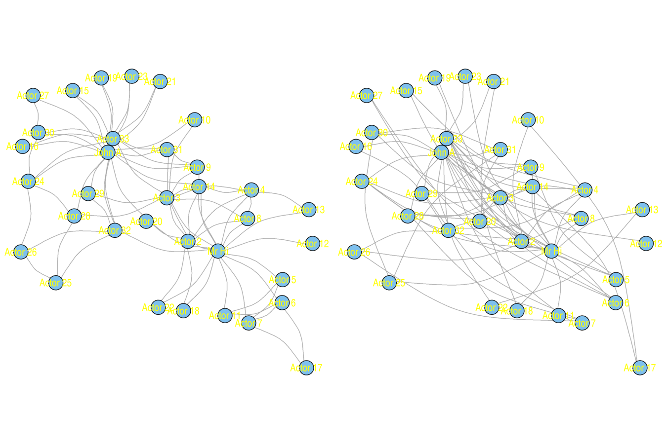
plot(eies.closefriends$t1)
Let's Indicate Attributes!
Scale vertex size by citations, color by discipline
library(RColorBrewer)library(compiler) my_ecdf_fun <- function(x.val, all.vals){ ret.val <- mean(x.val >= all.vals) return(ret.val) } my_ecdf_fun <- cmpfun(my_ecdf_fun)vsize <- sapply(V(eies.closefriends$t1)$Citations, my_ecdf_fun, all.vals = V(eies.closefriends$t1)$Citations) vsize <- 7.5 + 15 * vsizeeach.discipline <- unique(V(eies.closefriends$t1)$Discipline_Name) n.disciplines <- length(each.discipline) vcol <- brewer.pal(n.disciplines, name = "Accent") vcol <- vcol[match(V(eies.closefriends$t1)$Discipline_Name, each.discipline)]plot(eies.closefriends$t1, vertex.color = vcol, vertex.size = vsize, vertex.label.color = "black", vertex.label.family = "sans")
Defaults for a Much Larger Case
Inadvisable for a network this large
vcount(wikidat) # 7115 nodes
ecount(wikidat) # 103689 edges
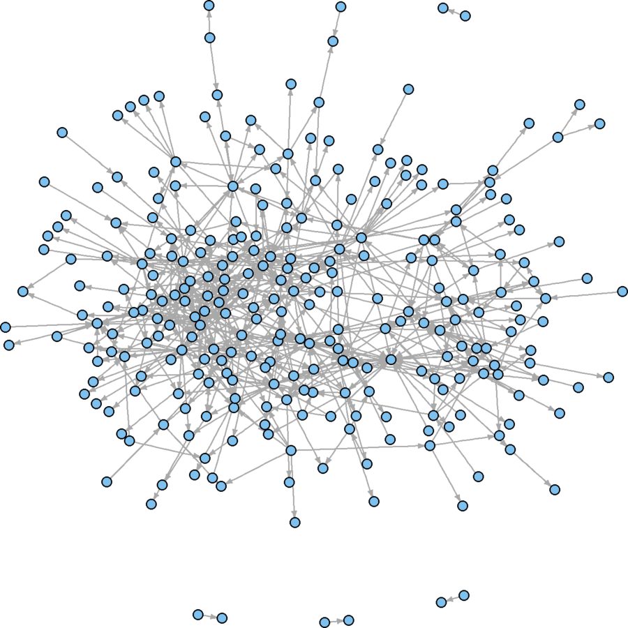
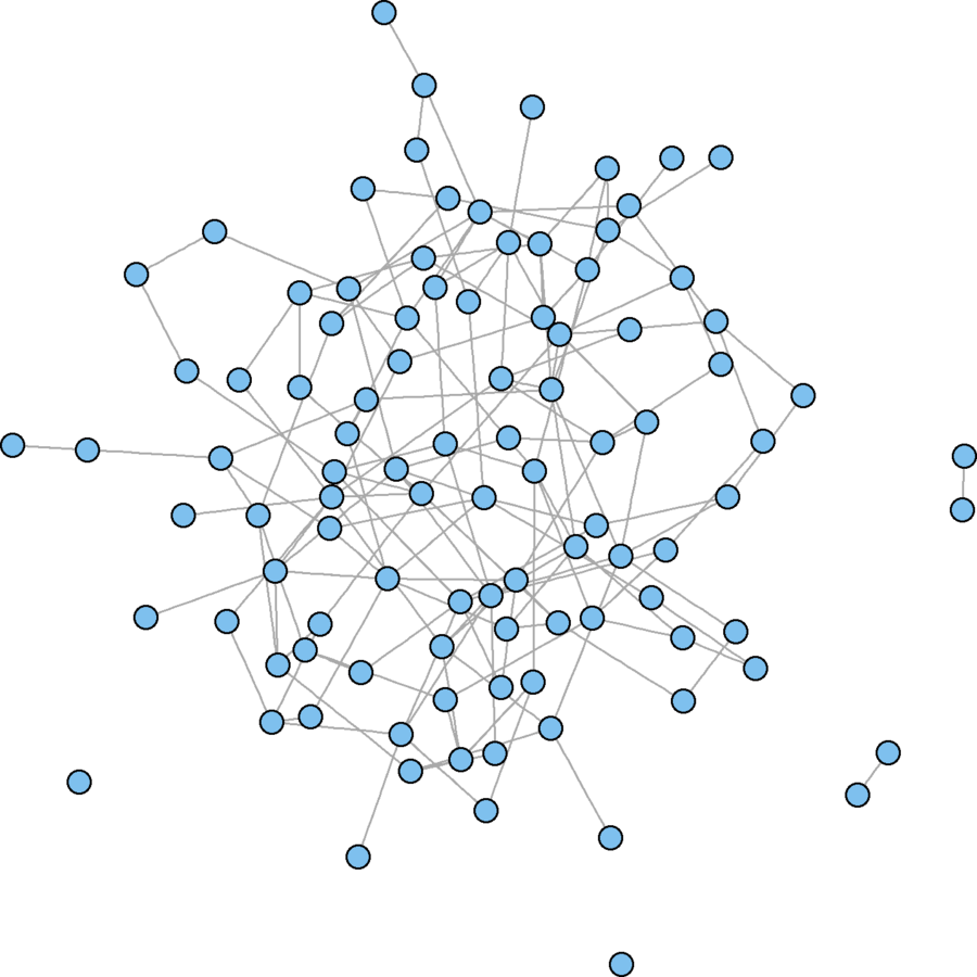
plot(wikidat)
What are the problems?
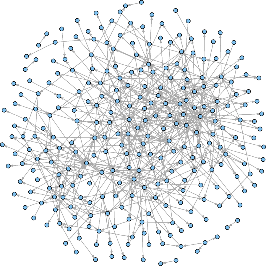
Subsample
Completely at Random
sampsize <- round(vcount(wikidat) * 0.05) # 5% sample
subsamp <- sample.int(vcount(wikidat), sampsize)
wikidat.sg <- induced.subgraph(wikidat, subsamp)
plot(wikidat.sg)
What are the problems?
Subsample
Completely at Random
sampsize <- round(vcount(wikidat) * 0.05) # 5% sample
subsamp <- sample.int(vcount(wikidat), sampsize)
wikidat.sg <- induced.subgraph(wikidat, subsamp)
plot(wikidat.sg)
- Nodes too large
- Labels don't provide information
plot(wikidat.sg, vertex.size = 3, vertex.label = "")
What are the problems?
Subsample
Visual problems
- Too many isolates
- Arrowheads too large
subsamp <- which(degree(wikidat.sg, mode = "all") > 0)
wikidat.sg <- induced.subgraph(wikidat.sg, subsamp)
plot(wikidat.sg, vertex.size = 3, vertex.label = "", edge.arrow.size = 0.5)
Much better, visually
But what are some conceptual problems using this technique?
Conceptual Problems with Random Sampling
- Grossly underrepresents degree
- Majority of alters absent
- Underestimates connectivity
- Conceptually naïve
- Sample could reflect structure
- Replication limitations
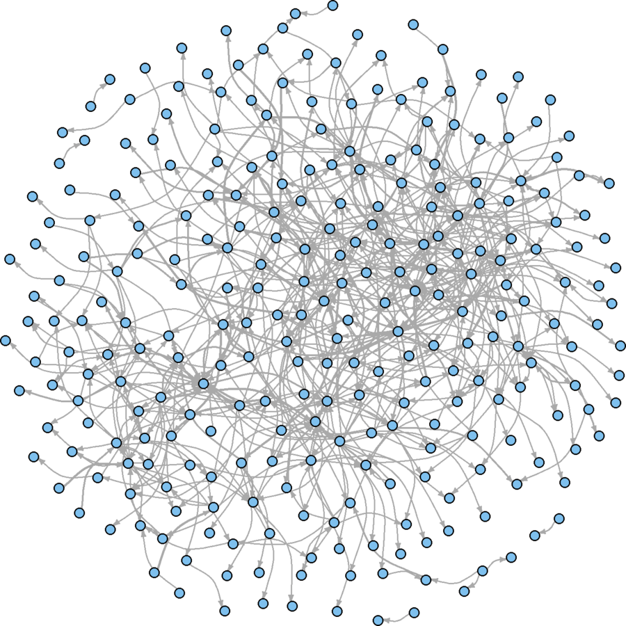
Alternative Subsampling Strategy
I want to portray communities and leadership
# Sample based on betweenness and large communities cond1 <- V(wikidat)$betw > 1 cond2 <- V(wikidat)$comms %in% c(3, 4, 5, 9, 11) subsamp <- which(cond1 & cond2) wikidat.sg <- induced.subgraph(wikidat, subsamp) vcount(wikidat.sg) # From 7,115 to 1,372 nodes ecount(wikidat.sg) # From 103,689 to 40,587 edges # Still too big to see anything. # Systematic 25% sample on eigenvector centrality evrank <- rank(V(wikidat.sg)$evcent, "random") nsyssamp <- seq(from = 1, to = max(evrank), by = 4) nsyssamp <- which(evrank%in% nsyssamp) wikidat.sg <- induced.subgraph(wikidat.sg, nsyssamp)# Systematic 25% sample on edge betweenness ebrank <- rank(E(wikidat.sg)$eb, "random") esyssamp <- seq(from = 1, to = max(ebrank), by = 4) esyssamp <- which(ebrank %in% esyssamp) wikidat.sg <- subgraph.edges(wikidat.sg, esyssamp) plot(wikidat.sg, vertex.size = 3, vertex.label = "", edge.arrow.size = 0.25)
Not too bad!
Layout
There are many layout algorithms out there
Their default values compromise between quality and efficiency
?layout.auto
wikidat.sg.lo <- layout.fruchterman.reingold(wikidat.sg, params = list(niter = 2500, area = vcount(wikidat.sg)^3))
V(wikidat.sg)$x <- wikidat.sg.lo[,1]
V(wikidat.sg)$y <- wikidat.sg.lo[,2]
plot(wikidat.sg, vertex.size = 3, vertex.label = "", edge.arrow.size = 0.25)
Better use of space, but hairballish
What are your empirical interests?
-
Sizes
- Colors and shading
- Categorical variables
- Interval and ordinal variables
- Transparency
Parameters to Vary
- Nodes
- Non-continuous: Shape, node color, border color
- Continuous: Node size, border width, color
- Edges
- Non-continuous: Color, line type, arrowhead type
- Continuous: Width, color
- Labels: Size, color, visibility
Edge Adjustments
Emphasize those with higher betweenness
Use width to convey it
ewidth <- sapply(E(wikidat.sg)$eb, my_ecdf_fun, E(wikidat.sg)$eb)
E(wikidat.sg)$width <- (1.25 * ewidth)^2
plot(wikidat.sg, vertex.size = 3, vertex.label = "", edge.arrow.size = 0.25, edge.curved = TRUE)
Only a slight improvement
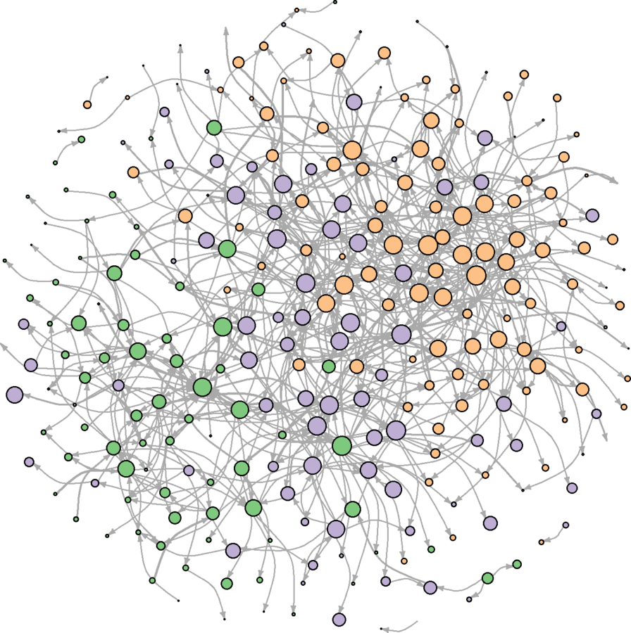
Node Adjustments
Color by community
Scale by eigenvector centrality
vcols <- brewer.pal(3, "Accent")
names(vcols) <- unique(V(wikidat.sg)$comms)
V(wikidat.sg)$color <- vcols[as.character(V(wikidat.sg)$comms)]
V(wikidat.sg)$size <- 6 * sapply(V(wikidat.sg)$evcent, my_ecdf_fun, V(wikidat.sg)$evcent)
plot(wikidat.sg, vertex.label = "", edge.arrow.size = 0.25, edge.curved = TRUE)
Communities better portrayed
Additional Sweep
Halve the number of edges
Same technique as before
ebrank <- rank(E(wikidat.sg)$eb, "random")
esyssamp <- seq(from = 1, to = max(ebrank), by = 2)
esyssamp <- which(ebrank %in% esyssamp)
wikidat.sg <- subgraph.edges(wikidat.sg, esyssamp)
plot(wikidat.sg, vertex.label = "", edge.arrow.size = 0.25, edge.curved = .25)
Much more clear
Do the main observations hold across different layouts?
par(mfrow = c(2, 2), mar = c(0.1, 0.1, 0.1, 0.1))
plot(wikidat.sg, vertex.label = "", edge.arrow.size = 0.25, edge.curved = .25, layout = layout.kamada.kawai, margin = c(0, 0, 0, 0))
plot(wikidat.sg, vertex.label = "", edge.arrow.size = 0.25, edge.curved = .25, layout = layout.circle, margin = c(0, 0, 0, 0))
plot(wikidat.sg, vertex.label = "", edge.arrow.size = 0.25, edge.curved = .25, layout = layout.svd, margin = c(0, 0, 0, 0))
plot(wikidat.sg, vertex.label = "", edge.arrow.size = 0.25, edge.curved = .25, layout = layout.mds, margin = c(0, 0, 0, 0))

Color Edges by Community
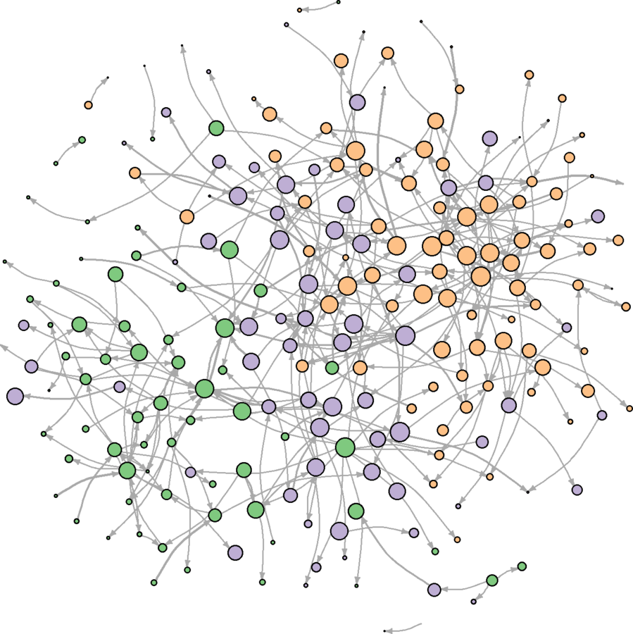
wikidat.sg.elist <- get.edgelist(wikidat.sg, names = FALSE)
edgecolor <- apply(wikidat.sg.elist, 1, function(x){
    c1 <-V(wikidat.sg)$comms[x[1]]
    c2 <- V(wikidat.sg)$comms[x[2]]
    return(ifelse(c1 == c2, vcols[as.character(c1)], "darkgrey"))
    })
E(wikidat.sg)$color <- edgecolordev.off()
plot(wikidat.sg, vertex.label = "", edge.arrow.size = 0.25, edge.curved = .25, layout = layout.svd, margin = c(0, 0, 0, 0))
Advice
- Less is more
- Fewer modifications are better than more
- Smaller data is easier to represent than larger data
- Transparency when reporting visualization
- Informative and intuitive over beautiful
- Practical over gimmicky
- Science over art
For more options, see
?igraph.plottingGraph-Level Indices
Graph-Level Indices
Some custom commands
(May take a few minutes)
source("http://pastebin.com/raw.php?i=SErkr5sg")- ei_index
- transitivity_directed
- uman_game
- rewire_dyads
Graph-Level Indices
What's the edgewise reciprocity for Wikipedia administrator voting?
reciprocity(wikidat)5.6% of all edges are reciprocated
Is this figure big or small?
Bigger or smaller than what?
We need to establish a basis for comparison.
Graph-Level Indices
Affected by network size and density
Example
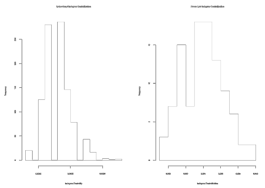
graph.order <- seq(from = 10, to = 100, by = 5)
graph.trans <- sapply(graph.order, function(x) replicate(1000, transitivity(erdos.renyi.game(x, .1))))
graph.apl <- sapply(graph.order, function(x) replicate(1000, average.path.length(erdos.renyi.game(x, .1))))
par(mfrow = c(1, 2))
plot(x = graph.order, y = apply(graph.trans, 2, mean), ylim = c(0, 1), xlim = c(0, 100), type = "l", xlab = "Order", ylab = "Transitivity", main = "Tie Prob = 0.10; Simulations=1000")
lines(x = graph.order, y = apply(graph.trans, 2, quantile, probs = .025, na.rm = TRUE), col = "red", lty = 2, type = "l")
lines(x = graph.order, y = apply(graph.trans, 2, quantile, probs = .975, na.rm = TRUE), col = "red", lty = 2, type = "l")
plot(x = graph.order, y = apply(graph.apl, 2, mean), ylim = c(0, 5), xlim = c(0, 100), type = "l", xlab = "Order", ylab = "Average Path Length", main = "Tie Prob = 0.10; Simulations = 1000")
lines(x = graph.order, y = apply(graph.apl, 2, quantile, probs = .025, na.rm = TRUE), col = "red", lty = 2, type = "l")
lines(x = graph.order, y = apply(graph.apl, 2, quantile, probs = .975, na.rm = TRUE), col = "red", lty = 2, type = "l")
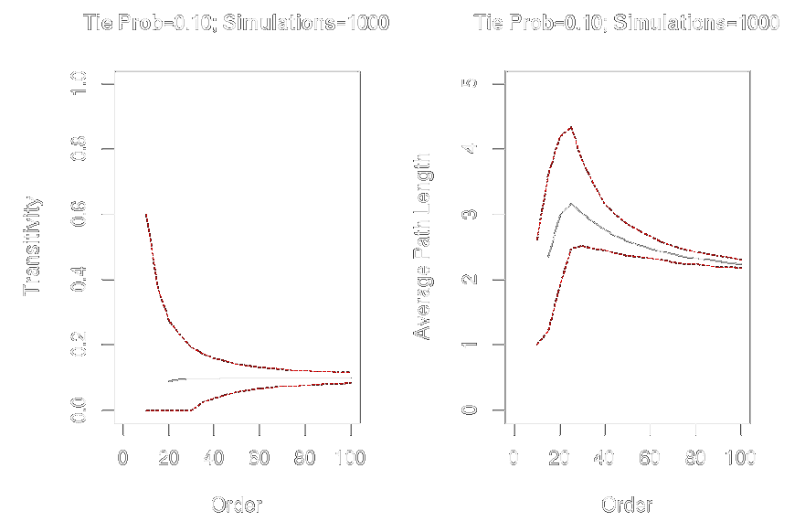
Graph-Level Indices
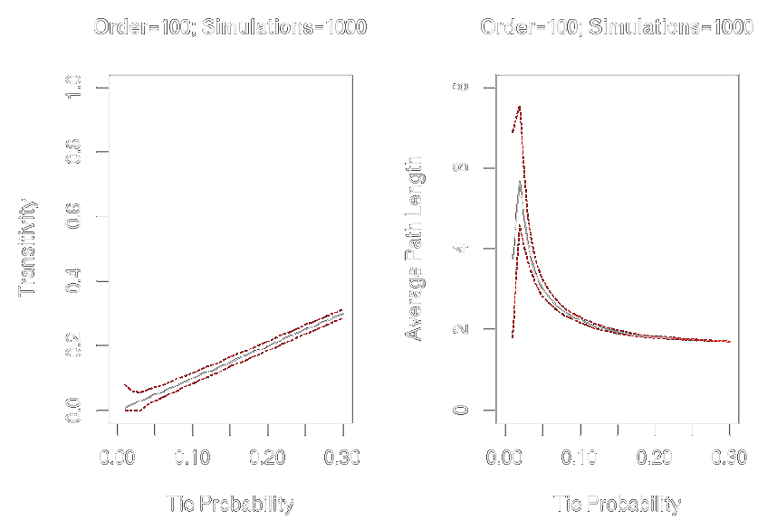
Affected by network size and density
graph.tieprob <- seq(from = .01, to = .30, by = .01)graph.trans <- sapply(graph.tieprob, function(x) replicate(1000, transitivity(erdos.renyi.game(100, x))))graph.apl <- sapply(graph.tieprob, function(x) replicate(1000, average.path.length(erdos.renyi.game(100, x))))par(mfrow = c(1, 2))plot(x = graph.tieprob, y = apply(graph.trans, 2, mean), ylim = c(0, 1), xlim = c(0, .3), type = "l", xlab = "Tie Probability", ylab = "Transitivity", main = "Order = 100; Simulations = 1000")lines(x = graph.tieprob, y = apply(graph.trans, 2, quantile, probs = .025, na.rm = TRUE), col = "red", lty = 2, type = "l")lines(x = graph.tieprob, y = apply(graph.trans, 2, quantile, probs = .975, na.rm = TRUE), col = "red", lty = 2, type = "l")plot(x = graph.tieprob, y = apply(graph.apl, 2, mean), ylim = c(0,8), xlim = c(0,.3), type = "l", xlab = "Tie Probability", ylab = "Average Path Length", main = "Order=100; Simulations = 1000")lines(x = graph.tieprob, y = apply(graph.apl, 2, quantile, probs = .025, na.rm = TRUE), col = "red", lty = 2, type = "l")lines(x = graph.tieprob, y = apply(graph.apl, 2, quantile, probs = .975, na.rm = TRUE), col = "red", lty = 2, type = "l")
Random Graph Comparisons
Conditional Uniform Graph (CUG) test
- Measure observed statistic on a graph
- Generate many random graphs (~1000)
- Take the same measurement from each
- Compare the observed statistic to the random ones
Two families
- Reassignment methods
- Graph generators
Reassignment Methods
"Shuffling" ties and attributes
- Permutation tests
- Rewiring tests
Permutation tests
- Permute an attribute to test its relationship to a nodal property
- Permute a graph to test its relationship to another graph
# Do conservative blogs have more links than liberal ones? polblogs <- nexus.get(id = "polblogs") #0 = liberal, 1 = conservative polblogs.totdeg <- degree(polblogs, mode = "all") obs.diff <- mean(polblogs.totdeg[V(polblogs)$LeftRight == 1]) - mean(polblogs.totdeg[V(polblogs)$LeftRight == 0]) perm.fun <- function(){ perm.attribs <- sample(V(polblogs)$LeftRight) return(mean(polblogs.totdeg[perm.attribs == 1]) - mean(polblogs.totdeg[perm.attribs == 0])) }; perm.fun<-cmpfun(perm.fun)exp.diffs <- replicate(1000, perm.fun()) mean(obs.diff > exp.diffs) # ~0.86, not significantly greater than by chance assignment
"Why not just use a t-test?"
Permutation tests
E-I Index (Krackhardt and Robert Stern 1988)
(Outgroup Ties - Ingroup Ties) / Total Ties
obs.val <- ei_index(polblogs, V(polblogs)$LeftRight)
exp.val <- replicate(1000, ei_index(polblogs, sample(V(polblogs)$LeftRight)))
mean(obs.val < exp.val) # We expect fewer outgroup ties
Permutation Tests
EI Index = (Outgroup Ties - Ingroup Ties) / Total Ties
# Friendship homophily by discipline among researchers# Time 1 obs.val.t1 <- ei_index(eies.closefriends$t1, V(eies.closefriends$t1)$Discipline_Name) exp.val.t1 <- replicate(1000, ei_index(eies.closefriends$t1, sample(V(eies.closefriends$t1)$Discipline_Name)))# Time 2 obs.val.t2 <- ei_index(eies.closefriends$t2, V(eies.closefriends$t2)$Discipline_Name) exp.val.t2 <- replicate(1000, ei_index(eies.closefriends$t2, sample(V(eies.closefriends$t2)$Discipline_Name)))# Compare the homophily effect & its non-random probability c(t1 = obs.val.t1, t1.p = mean(obs.val.t1 < exp.val.t1), t2 = obs.val.t2, mean(obs.val.t2 < exp.val.t2))
Rewiring tests
One of two approaches
- Shuffle edges (or dyads)
- Shuffle edge weights
Preserves degree (and edge weight) distribution
karate <- nexus.get("karate")
karate.lo <- layout.kamada.kawai(karate, params = list(niter = 1000))

par(mfrow = c(1, 2))
plot(karate, vertex.size = 5, vertex.label = V(karate)$name, vertex.label.family = "sans", margin = c(0, 0, 0, 0), edge.curved = .33, layout = karate.lo)

karate.rw <- rewire(karate, mode = "simple", niter = 10*ecount(karate))
plot(karate.rw, vertex.size = 5, vertex.label = V(karate)$name, vertex.label.family = "sans", margin = c(0, 0, 0, 0), edge.curved = .33, layout = karate.lo)
Original (left) and Rewired (right)
Rewired Transitivity
obs.trans <- transitivity(karate)karate.rw.fun <- function(){krw <- rewire(karate, mode = "simple", niter = 10 * ecount(karate))return(transitivity(krw))}; karate.rw.fun <- cmpfun(karate.rw.fun)exp.trans <- replicate(1000, karate.rw.fun())mean(obs.trans > exp.trans) # ~0.87
What's the interpretation of this finding?
Rewired Transitivity
Is the transitivity in this directed network greater than chance?
Did it increase from the first to second time point?
Rewired dyads control for reciprocity and degree distribution
n.researchers <- vcount(eies$t1) n.rewires <- 10 * n.researchers * (n.researchers - 1) obs.val.t1 <- transitivity_directed(eies$t1) obs.val.t2 <- transitivity_directed(eies$t2) # Will take some time. # Would recommend at least 1000, not 250, replicationsexp.val.t1 <- replicate(250, transitivity_directed(rewire_dyads(eies$t1, n.rewires))) exp.val.t2 <- replicate(250, transitivity_directed(rewire_dyads(eies$t2, n.rewires)))c(t1 = obs.val.t1, t1.p = mean(obs.val.t1 > exp.val.t1), t2 = obs.val.t2, t2.p = mean(obs.val.t2 > exp.val.t2))
Graph Generators
- Erdős–Rényi model
- Power Law model
- Watts and Strogatz model
- Exponential random graph models
- ...and many others
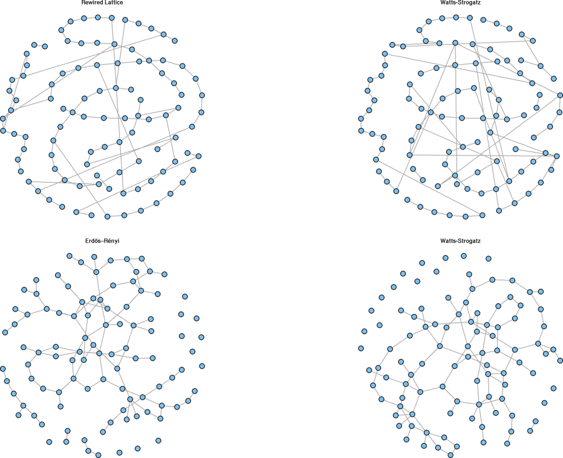
Erdős–Rényi model
A fixed number (or proportion) of edges are randomly assigned to a fixed set of nodes.
Variants
- Exact #ties or density
- Directed, undirected
- Dyad census-conditioned
er.graph <- erdos.renyi.game(100, .03)
plot(er.graph, vertex.size = 5, vertex.label = "")
obs.incent <- centralization.degree(wikidat, mode = "in", loops = FALSE)$centralization
exp.incent.fun <- function(){
  new.net <- erdos.renyi.game(vcount(wikidat), ecount(wikidat), type = "gnm", directed = TRUE)
  return(centralization.degree(new.net, mode = "in", loops = FALSE)$centralization)
  }; exp.incent.fun <- cmpfun(exp.incent.fun)
exp.incent <- replicate(1000, exp.incent.fun())
mean(obs.incent > exp.incent)
Erdős–Rényi model
obs.incent <- centralization.degree(wikidat, mode = "in", loops = FALSE)$centralization exp.incent.fun.ec <- function(){ new.net <- erdos.renyi.game(vcount(wikidat), ecount(wikidat), type = "gnm", directed = TRUE) return(centralization.degree(new.net, mode = "in", loops = FALSE)$centralization) }; exp.incent.fun.ec <- cmpfun(exp.incent.fun.ec) exp.incent.ec <- replicate(500, exp.incent.fun.ec()) c(obs = obs.incent, exp.ec = mean(obs.incent > exp.incent.ec))# An alternative model that will take too much time # Set sparse = TRUE if you don't have much RAM exp.incent.fun.dc <- function(){ dc <- unlist(dyad.census(wikidat)) new.net <- uman_game(vcount(wikidat), dc, sparse = FALSE) return(centralization.degree(new.net, mode = "in", loops = FALSE)$centralization) }; exp.incent.fun.dc <- cmpfun(exp.incent.fun.dc) exp.incent.dc <- replicate(500, exp.incent.fun.dc())
Erdős–Rényi model
Power Law model
Assumptions
Networks grow according to the principle of preferential attachment.
P(X=x) ~ x^(-alpha)
Nodes are of degree greater than or equal to x
P(X=x) is the probability of observing a node with degree x or greater
alpha is the scalar
(Barabási and Albert 1999)
Power Law model
wikidat.in <- degree(wikidat, mode = "in")
wikidat.out <- degree(wikidat, mode = "out")
wikidat.plfit.in <- power.law.fit(wikidat.in)
wikidat.plfit.out <- power.law.fit(wikidat.out)
print(c(wikidat.plfit.in$alpha, wikidat.plfit.out$alpha))
exp.incent.pl.fun <- function(){
  new.net <- static.power.law.game(vcount(wikidat), ecount(wikidat), exponent.out = wikidat.plfit.out$alpha, exponent.in = wikidat.plfit.in$alpha)
  return(centralization.degree(new.net, mode="in", loops = FALSE)$centralization)
  }; exp.incent.pl.fun <- cmpfun(exp.incent.pl.fun)
exp.incent.pl <- replicate(500, exp.incent.pl.fun())
mean(obs.incent > exp.incent.pl) # Obs more centralized
par(mfrow = c(1, 2))
hist(exp.incent.ec, main = "E-R Indegree Centralization")
hist(exp.incent.pl, main = "Power Law Indegree Centralization") # ~10x more centralized graphs
Watts and Strogatz model
Assumptions
Local neighborhoods bridged by a few actors with ties that jump across neighborhoods.
Game
-
Begin with a lattice
- Each actor initially has the same degree, neighborhood index (nei) * 2
-
Rewire with a probability of
p
par(mfrow=c(1, 2))
g1 <- graph.lattice(100, nei = 1)# nei = mean degree / 2
g1.layout<-layout.fruchterman.reingold(g1)
V(g1)$x <- g1.layout[ , 1]; V(g1)$y <- g1.layout[ , 2]
g1.rewire <- rewire.edges(g1, p = 0.1) # prob of .1 rewire
plot(g1, vertex.size = 5, vertex.label = "", main = "Lattice")
plot(g1.rewire, vertex.size = 5, vertex.label = "", main = "Rewire")
Watts and Strogatz model
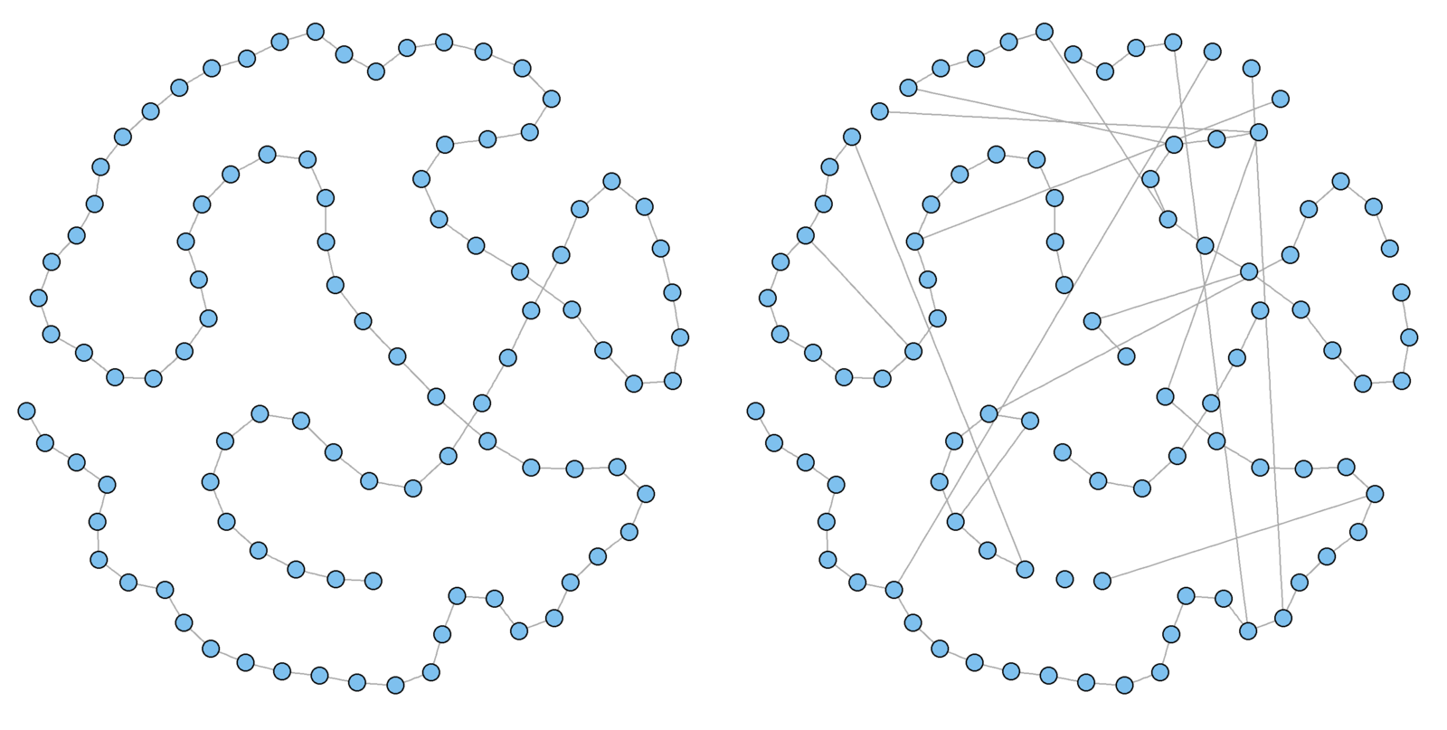
Watts and Strogatz model
Question
What's the relationship between the neighborhood index (nei) and graph density?
Watts and Strogatz model
Low values for p resemble lattices
#The following two plots should be approximately equal
dev.off(); par(mfrow = c(1, 2))
sw.net <- watts.strogatz.game(dim = 1, size = 100, nei = 1, p = .1)
plot(g1.rewire, vertex.size = 5, vertex.label = "", main = "Rewired Lattice")
plot(sw.net, vertex.size = 5, vertex.label = "", layout = g1.layout, main = "Watts-Strogatz")
High values for
p
become closer to Erdős–Rényi graphs
par(mfrow = c(1, 2))
g2.ws <- watts.strogatz.game(dim = 1, size = 100, nei = 1, p = .9)
g2.er <- erdos.renyi.game(100, (2 * 100 / 2) / (100 * 99 / 2), directed = FALSE)
plot(g2.ws, vertex.size = 5, vertex.label = "", main = "Watts-Strogatz")
plot(g2.er, vertex.size = 5, vertex.label = "", main = "Erdős–Rényi")
Rewiring Demonstration
Exponential random graph models
Exercises
Recreate the first two plots in this lab using the Watts and Strogatz model. Fix the order (size) to 100 and set the density to approximately 0.02. Vary p from 0 to 1 by .01.
(Hint: mean degree equals the number of edges divided by the number of nodes.)
Recreate the power law exercise on degree centralization for the political blog network. If appropriate to model as a power law, is this network more centralized than predicted?
Two-Mode Networks
Two-Mode Networks are Special
- Clustering follows a different mechanism
- Distance can take on a different meaning
- Depends upon conceptualization of tie strength
Traditionally "projected" as a one-mode network.
- Theoretical problems
- Assumes an "event" creates ties among all participating actors
- Do you always know everyone at each party you attend?
- Some actors and events are much more inclusive
- Should their relationships hold the same weight?
- Methodological problems
- Creates a complete subgraph ("clique") around each event
- Increases density
Two-Mode Network Software
-
Limited functions in igraph (R, Python, C, Ruby)
-
More capabilities in tnet (R)
-
NetworkX (Python)
library(igraph)
library(tnet)
library(compiler)
marvnet <- read.graph("http://bioinfo.uib.es/~joemiro/marvel/porgat.txt", format = "pajek")
V(marvnet)$name <- V(marvnet)$id
marvnet.tnet <- get.edgelist(marvnet, names = FALSE)
marvnet.tnet <- as.tnet(marvnet.tnet, type = "binary two-mode tnet")
Two-Mode Network Software
-
Limited functions in igraph (R, Python, C, Ruby)
- More capabilities in tnet (R) and NetworkX (Python)
download.file("https://raw.githubusercontent.com/kjhealy/revere/master/data/PaulRevereAppD.csv", "PaulRevere.csv", method = "wget")
amrev <- read.csv("PaulRevere.csv", row.names = 1)
file.remove("PaulRevere.csv")
amrev.el <- which(amrev == 1, arr.ind = TRUE)
amrev.el[, 1] <- rownames(amrev)[as.numeric(amrev.el[, 1])]
amrev.el[, 2] <- colnames(amrev)[as.numeric(amrev.el[, 2])]
amrev <- graph.data.frame(amrev.el, directed = FALSE)
V(amrev)$type <- V(amrev)$name %in% amrev.el[, 2]
Convert it to tnet
amrev.tnet <- get.edgelist(amrev, names = FALSE)
amrev.tnet <- as.tnet(amrev.tnet, type = "binary two-mode tnet")
Clustering Coefficient
Closed Three-Paths (Robins and Alexander [2004])
ra_clust <- function(g){
    g.motif <- graph.motifs(g, size = 4)
    threepaths <- g.motif[7]
    fourcycles <- 4 * g.motif[9]
    ret.val <- fourcycles / (fourcycles + threepaths)
    return(ret.val)
    }
ra_clust <- cmpfun(ra_clust)

amrev.raclust <- ra_clust(amrev)
amrev.raclust
# Much slower, but faster version available (email Opsahl)
amrev.oclust <- clustering_tm(amrev.tnet)
amrev.oclust
Local Clustering Coefficient
Robins and Alexander (2004)
local_ra_clust <- function(g, vind){ new.g <- graph.neighborhood(g, order = 2, nodes = vind)[[1]] new.g.motif <- graph.motifs(new.g, size = 4) threepaths <- new.g.motif[7] fourcycles <- 4 * new.g.motif[9] retval <- ifelse(fourcycles + threepaths > 0, fourcycles / (fourcycles + threepaths), NaN)return(retval) } local_ra_clust <- cmpfun(local_ra_clust) amrev.raclust.loc <- sapply(1:vcount(amrev), local_ra_clust, g = amrev)
(Took my computer ~4 minutes)
amrev.oclust.loc <- clustering_local_tm(amrev.tnet)Local Clustering Coefficient
Robins and Alexander (2004)
Whose Ego Networks Had the Highest Clustering?
# Identify both the actors and those actors with valid clustering coefficients
amrev.raclust.loc.actors.ind <- which(is.nan(amrev.raclust.loc[which(V(amrev)$type == FALSE)]) == FALSE)
amrev.raclust.loc.actors <- data.frame(name = V(amrev)$name[amrev.raclust.loc.actors.ind])
amrev.raclust.loc.actors$clust <- amrev.raclust.loc[amrev.raclust.loc.actors.ind]
amrev.raclust.loc.actors$rank <- rank(amrev.raclust.loc.actors$clust)
amrev.raclust.loc.actors[order(amrev.raclust.loc.actors$clust, amrev.raclust.loc.actors$name), ]
Randomization
Two main options
- Random network generation
- Edge rewires
# Generate a random network with the same parameters as the Marvel network
n.primary <- sum(V(marvnet)$type == FALSE)
n.secondary <- vcount(marvnet) - n.primary
marvnet.rand.el <- rg_tm(ni = n.primary, np = n.secondary, ties = ecount(marvnet))
head(marvnet.rand.el) # It's an edgelist.
# Export it to igraph
summary(marvnet.rand.el)
# Because both the first and second mode begin at 1 ...
marvnet.rand.el[, "p"] <- marvnet.rand.el[, "p"] + n.primary
marvnet.rand.type <- c(rep(FALSE, times = n.primary), rep(TRUE, times = n.secondary))
marvnet.rand.atts <- data.frame(name = 1:vcount(marvnet), type = marvnet.rand.type)
marvnet.rand <- graph.data.frame(marvnet.rand.el, directed = FALSE, vertices = marvnet.rand.atts)Randomization
Let's compare the degree distributions. First mode
par(mfrow = c(2, 2))
tempdegree <- degree(marvnet, v = which(V(marvnet)$type == FALSE))
hist(log(1 + tempdegree), main = "Observed", xlab = "Issues in Which Each Character Appears (log)", ylab = "Frequency")
tempdegree <- degree(marvnet.rand, v = which(V(marvnet)$type == FALSE))
hist(log(1 + tempdegree), main = "Random", xlab = "Issues in Which Each Character Appears (log)", ylab = "Frequency")
tempdegree <- degree(marvnet, v = which(V(marvnet)$type == TRUE))
hist(log(1 + tempdegree), main = "Observed", xlab = "Characters Appearing in Each Issue (log)", ylab = "Frequency")
tempdegree <- degree(marvnet.rand, v = which(V(marvnet)$type == TRUE))
hist(log(1 + tempdegree), main = "Random", xlab = "Characters Appearing in Each Issue (log)", ylab = "Frequency")
Randomization
Random graph generator
-
Good for small, dense networks
- Highly general
- Controls for size and density
- Does not control for degree distribution
# tnet method. # Do not use now, as it will take A VERY LONG TIME. # Also allows for weighted two-mode data and can shuffle weightsamrev.rand.rw <- rg_reshuffling_tm(amrev.tnet) # Reshuffles each edge
Randomization
Rewiring method
# igraph method. Inadviseable for large networks# First, recreate the bipartite network, but treat it as directed to preserves the bipartite structure # Second, rewire the directed two-mode network # Third, remove the directionrewire_tm <- function(g, niter = NULL){ g.el <- get.edgelist(g) new.g <- graph.data.frame(g.el, directed = TRUE) V(new.g)$type <- V(g)$type nswaps <- ifelse(is.null(niter), 10 * ecount(g), niter) new.g <- rewire(new.g, mode = "simple", nswaps) new.g <- as.undirected(new.g) return(new.g) } rewire_tm <- cmpfun(rewire_tm)
amrev.raclust.exp <- replicate(1000, ra_clust(rewire_tm(amrev)))
summary(amrev.raclust.exp)
mean(amrev.raclust > amrev.raclust.exp)Graph-Level Indices
When measuring graph-level indices on a projected network....
- Project observed two-mode data to one-mode
- Take graph-level measurement
- Simulate
- Simulate two-mode network from observed two-mode networks
- Project simulated two-mode to a one-mode network
- Take graph-level measurement on simulated one-mode network
- Repeat to create distribution
- Compare observed measurement to simulated distribution
DO NOT SIMULATE BASED ON ONE-MODE PROJECTION
Projection
Four methods
- Dichotomous (Brieger. 1974. Social Forces.)
- Sum (Brieger. 1974. Social Forces.)
- Weighted
- k threshold cut-off
- Newman. 2001. Phys Rev E.
- Collaboration weight penalized by number of collaborators
- Backbone
-
Convert vertex pairs to z-scores using frequency counts
- Set alpha cut-off
- Retain edges beyond cut-off (+/-)
- Ahn, Ahnert, Bagrow, & Barabási. 2011. Scientific Reports.
- Serrano, Boguñá, & Vespignani. 2009 PNAS.
- Demonstration: http://pastebin.com/UNi0ryG3
Projection
Dichotomous
# tnet marv.dichot <- projecting_tm(marvnet.tnet, method = "binary") # Takes me ~1.5 minutes head(marv.dichot, 15) # Performed on "primary" mode only# igraph. # Set 'which' to "true" for the other mode # Set it to "both" for a list of both projections marv.dichot <- bipartite.projection(marvnet, multiplicity = FALSE, which = "false")
Projection
Sum
# tnet marv.sum <- projecting_tm(marvnet.tnet, method = "sum") # Takes me ~1.5 minutes head(marv.sum, 15) # Performed on "primary" mode only # k-threshold >= 12 marv.k12 <- marv.sum[which(marv.sum$w >= 12), ]# igraph marv.sum <- bipartite.projection(marvnet, multiplicity = TRUE, which = "false") head(E(marv.sum)$weight, 20) # k-threshold >= 12 marv.k12 <- subgraph.edges(marv.sum, which(E(marv.sum)$weight >= 12), delete.vertices = FALSE)
Projection
Newman (2001)
newman.2m.fun <- function(g, type = FALSE){
    vdeg <- degree(g)
    vneigh <- neighborhood(g, order = 1)
    mode.which <- ifelse(type, "true", "false")
    proj1m <- bipartite.projection(g, multiplicity = TRUE, which = mode.which)
    vmatch <- match(V(proj1m)$name, V(g)$name)
    proj1m.el <- get.edgelist(proj1m, names = FALSE)
    ncollabs <- function(x){
        orig.i <- vmatch[x[1]]
        orig.j <- vmatch[x[2]]
        art.k <- vneigh[[orig.i]][which(vneigh[[orig.i]] %in% vneigh[[orig.j]])]
        art.degs <- sum(1 / (vdeg[art.k] - 1))
        return(art.degs)
        }
    E(proj1m)$newman.w <- apply(proj1m.el, 1, ncollabs)
    return(proj1m)
    }
newman.2m.fun <- cmpfun(newman.2m.fun)
marv.newman <- newman.2m.fun(marvnet) # Took me ~30 seconds
head(cbind(E(marv.newman)$weight, E(marv.newman)$newman.w), 20)
Projection
Meanings
- Dichotomous
- "Any commonality"
- Sum
- Weighted
- "Number of commonalities"
- k threshold cut-off
- "Any commonality beyond k"
- Newman (2001)
- "Probability of dyadic interaction"
- Backbone
- "Dyadic interaction far above (or below) 'chance'"
- "Chance" based upon the level of an individual's activity
Distance
Weights affect the interpretation of distance
- Dichotomous
- Simple: number of collaborations away
- Weighted (including Newman)
- Distance between adjacent vertices is 1 / edge weight
- Average path length may be less than 1!
- Normalization (Opsahl, Agneessens, and Skvoretz 2010)
- Divide the weights by the mean of all weights
- Then calculate distance
Distance
# Dichotomousshortest.paths(marv.newman, v = 1, to = 2, weights = rep(1, ecount(marv.newman))) # 3 # Summed weights shortest.paths(marv.newman, v = 1, to = 2, weights = E(marv.newman)$weight) # 4 shortest.paths(marv.newman, 1, 2, weight = E(marv.newman)$weight / mean(E(marv.newman)$weight)) # 1.18 # Newmanedges2keep <- which(is.infinite(E(marv.newman)$newman.w) == FALSE) marv.newman <- subgraph.edges(marv.newman, edges2keep, delete.vertices = FALSE) shortest.paths(marv.newman, v = 1, to = 2, weights = E(marv.newman)$newman.w) # 0.38 shortest.paths(marv.newman, v = 1, to = 2, weights = E(marv.newman)$newman.w / mean(E(marv.newman)$newman.w)) # 1.33
Plotting
- Symbols
- Primary mode: circular nodes
- Secondary modes: square nodes
- Layout
- Bipartite
- Primary mode to the left
- Secondary mode to the right
- Multidimensional layouts appropriate also
- Projected as one-mode
- Any of the conventional layouts
Plotting
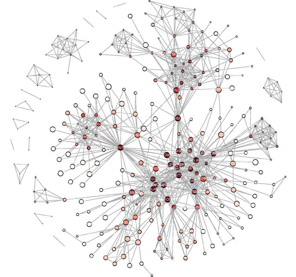
Marvel Universe Data
My inclinations
- Character co-appearance
- Project to one-mode
- Subsample
- Popular characters (two-mode degree)
- Strong relationships (Newman's weight)
- Remove isolates
- Clean the names
- Color by cohesion
- Scale vertices by closeness
- Scale edge widths by Newman's weight
Plotting
issues48 <- which((degree(marvnet) >= 48) & (V(marvnet)$type == FALSE))
issues48 <- which(V(marv.newman)$name %in% V(marvnet)$name[issues48])
marv.newman.sg <- induced.subgraph(marv.newman, issues48)
marv.newman.sg <- subgraph.edges(marv.newman.sg, which(E(marv.newman.sg)$newman.w > 4), delete.vertices = TRUE)
cleanupnames <- function(y){
    y <- strsplit(y, "/", fixed = TRUE)[[1]][1]
    y <- strsplit(y, " [", fixed = TRUE)[[1]][1]
    y <- gsub(".", "", y, fixed = TRUE)
    ylen <- nchar(y)
    lastchar <- substr(y, ylen, ylen)
    y <- ifelse(lastchar == " ", substr(y, 1, ylen - 1), y)
    return(y)
    }
cleanupnames <- cmpfun(cleanupnames)
V(marv.newman.sg)$name <- sapply(V(marv.newman.sg)$name, cleanupnames)
Plotting
library(RColorBrewer) # Community detection V(marv.newman.sg)$comm <- multilevel.community(marv.newman.sg, weights = E(marv.newman.sg)$weight)$membership max(V(marv.newman.sg)$comm) # 25 is too many communities to portray# k-cores V(marv.newman.sg)$kc <- graph.coreness(marv.newman.sg) kcmax <- max(V(marv.newman.sg)$kc) kcmax # 10 on a continuous scale is good. min(V(marv.newman.sg)$kc) # Because there are no isolates, minimum is 1. corecolors <- brewer.pal(max(V(marv.newman.sg)$kc), "Reds") corecolors <- c(rep("white", times = kcmax - 9), corecolors) V(marv.newman.sg)$color <- corecolors[V(marv.newman.sg)$kc]
Plotting
V(marv.newman.sg)$closeness <- closeness(marv.newman.sg, weights = E(marv.newman.sg)$weight / mean(E(marv.newman.sg)$weight), normalize = FALSE)
V(marv.newman.sg)$size <- ecdf(V(marv.newman.sg)$closeness)(V(marv.newman.sg)$closeness)
V(marv.newman.sg)$size <- V(marv.newman.sg)$size * 6
V(marv.newman.sg)$label.cex <- V(marv.newman.sg)$size / (4.5 * 2)
E(marv.newman.sg)$width <- ecdf(E(marv.newman.sg)$weight)(E(marv.newman.sg)$weight)g.lo <- layout.fruchterman.reingold(marv.newman.sg, params = list(niter = 2500, area = vcount(marv.newman.sg)^3))
V(marv.newman.sg)$x <- g.lo[ ,1]
V(marv.newman.sg)$y <- g.lo[ ,2]
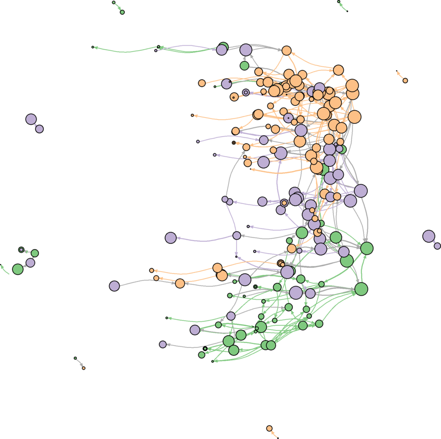
svg("MarvPlot.svg", height = 20, width = 20)
plot(marv.newman.sg, vertex.label.color = "black", vertex.label.family = "sans", margin = c(0, 0, 0, 0))
dev.off()
THANK YOU!
Benjamin Lind
blind@hse.ru
PDF:
R SNA Intro Lab St. Petersburg
By Benjamin Lind


.jpg)