Phase-Type Models in
Life Insurance

Dr Patrick J. Laub @ IME, München
Université Lyon 1

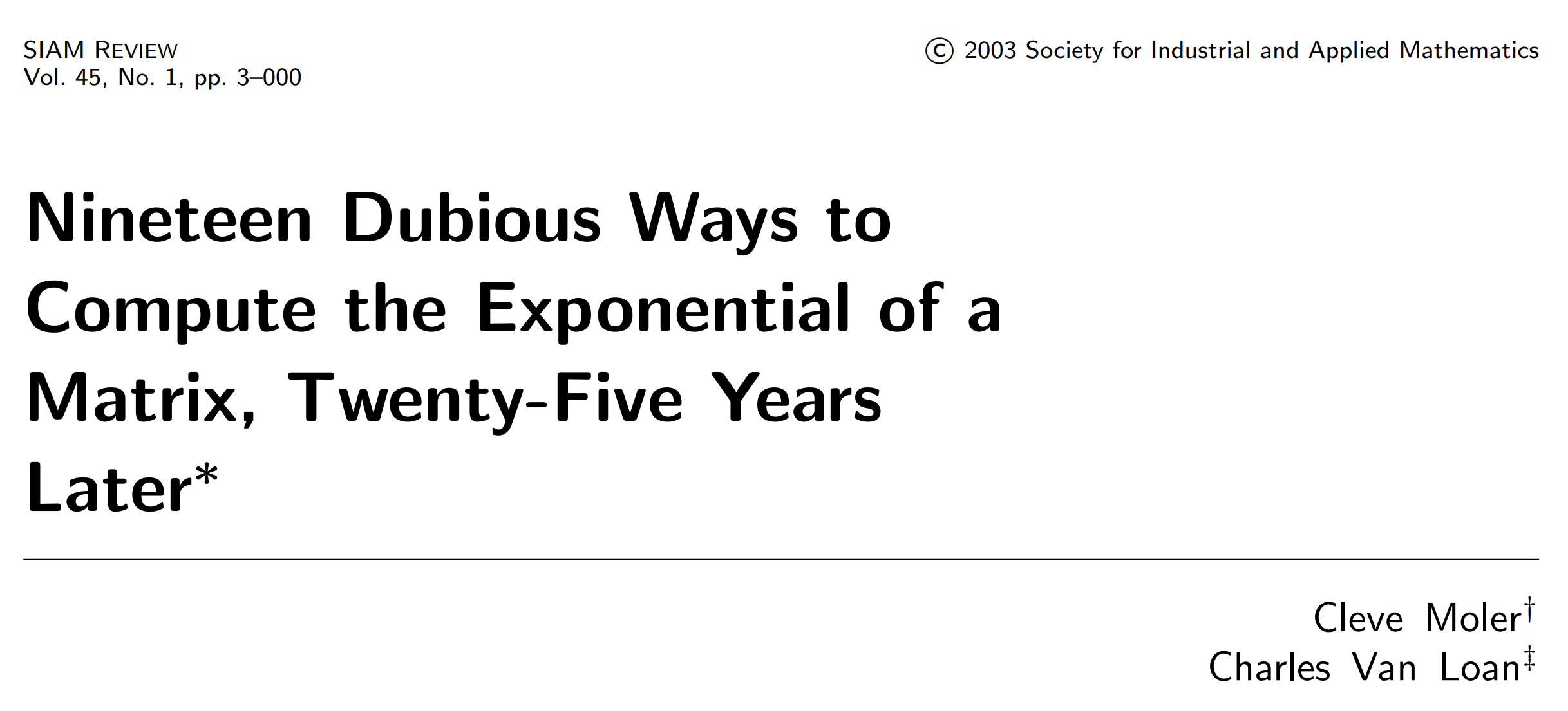
Motivating theory
Stochastic Models (2019), 34(4), 1-12.
Can read on https://arxiv.org/pdf/1803.00273.pdf
\tau
S_t
t
Guaranteed Minimum Death Benefit
S_\tau
\text{Payoff} = \max( S_{\tau}, K )
Equity-linked life insurance
\tau
t
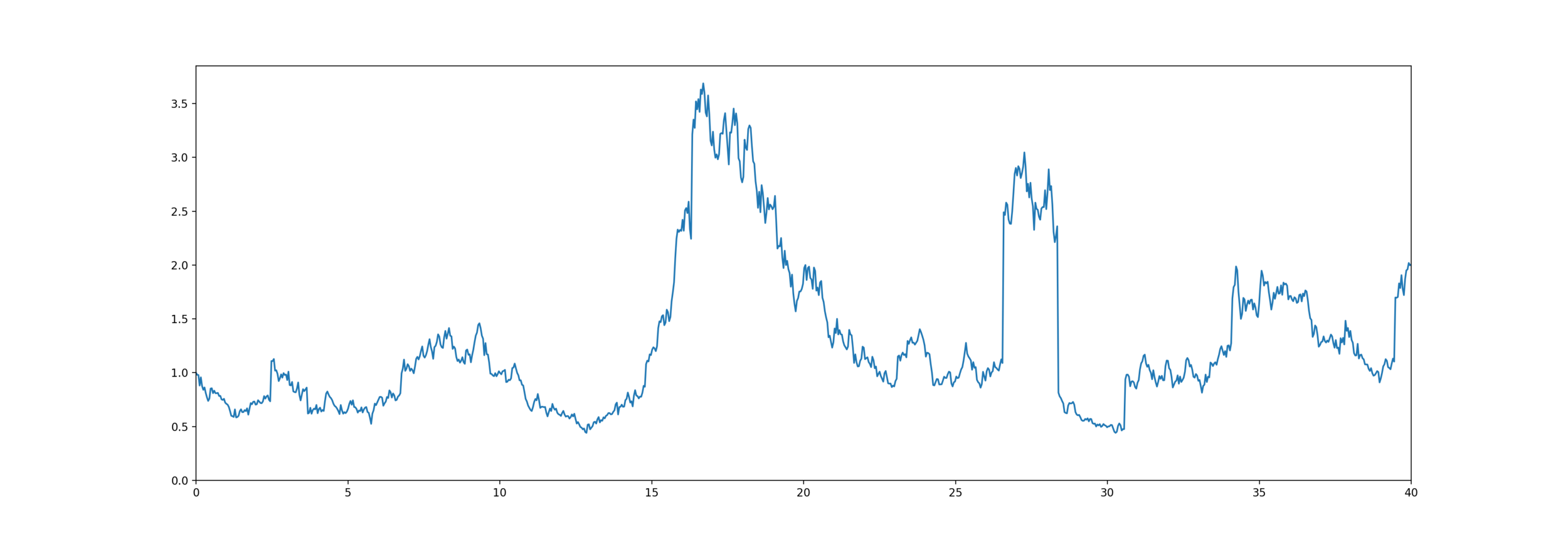
High Water Death Benefit
\text{Payoff} = \overline{S}_{\tau}
Equity-linked life insurance
\overline{S}_\tau
\overline{S}_t = \max_{s \le t} S_s
Model for mortality and equity
The customer lives for years,
\tau
\tau \sim \text{PhaseType}(\boldsymbol{\alpha}, \boldsymbol{T})
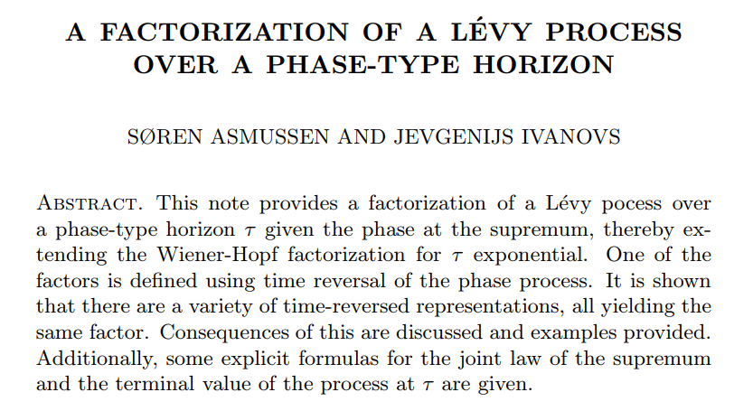
X_t \sim \text{Jump Diffusion}
S_t = S_0 \mathrm{e}^{X_t}
Equity is an exponential jump diffusion,
\text{Brownian Motion}(\mu, \sigma^2) + \text{Compound Poisson}(\lambda_1) + \text{Compound Poisson}(\lambda_2)
\text{Price} = \mathbb{E}[ \mathrm{e}^{-\delta \tau} \text{Payoff}( S_\tau, \overline{S}_\tau ) ]
S_t
t
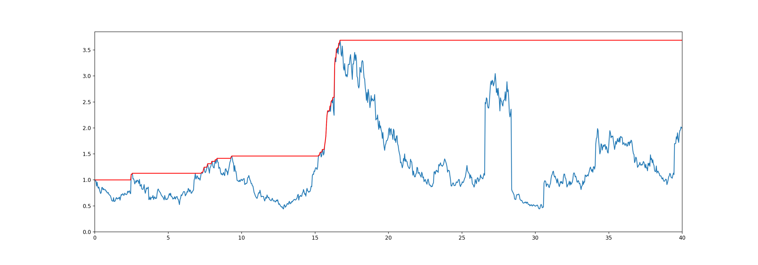
Exponential PH-Jump Diffusion
\text{UpJumpSize}_i \overset{\mathrm{i.i.d.}}{\sim} \text{PhaseType}(\boldsymbol{\alpha}_1, \boldsymbol{T}_1)
\text{DownJumpSize}_i \overset{\mathrm{i.i.d.}}{\sim} \text{PhaseType}(\boldsymbol{\alpha}_2, \boldsymbol{T}_2)
\# \text{UpJumps}(0, t) \sim \mathrm{Poisson}(\lambda_1 t)
\# \text{DownJumps}(0, t) \sim \mathrm{Poisson}(\lambda_2 t)
Get some helpful matrices
\boldsymbol{U} = \boldsymbol{U}(\delta, \mu, \sigma^2, \boldsymbol{\alpha}, \boldsymbol{T}, \lambda_1, \boldsymbol{\alpha}_1, \boldsymbol{T}_1, \lambda_2, \boldsymbol{\alpha}_2, \boldsymbol{T}_2 )
\text{UpJumpSize}_i \overset{\mathrm{i.i.d.}}{\sim} \text{PhaseType}({ \color{red} \boldsymbol{\alpha}_1 }, { \color{red} \boldsymbol{T}_1 })
\text{DownJumpSize}_i \overset{\mathrm{i.i.d.}}{\sim} \text{PhaseType}( { \color{red} \boldsymbol{\alpha}_2 }, { \color{red} \boldsymbol{T}_2 })
\# \text{UpJumps}(0, t) \sim \mathrm{Poisson}({ \color{red} \lambda_1 } t)
\# \text{DownJumps}(0, t) \sim \mathrm{Poisson}({ \color{red} \lambda_2 } t)
\text{Brownian Motion}({ \color{red} \mu }, { \color{red} \sigma^2 })
\tau \sim \text{PhaseType}({ \color{red} \boldsymbol{\alpha} }, { \color{red} \boldsymbol{T} })
\text{Price} = \mathbb{E}[ \mathrm{e}^{-{\color{red} \delta} \tau} \text{Payoff}( S_\tau, \overline{S}_\tau ) ]
\boldsymbol{U}_{n+1} = f(\boldsymbol{U}_n)
Use fixed-point approximation
\boldsymbol{U}^* = \boldsymbol{U}^*(\delta, \mu, \sigma^2, \boldsymbol{\alpha}, \boldsymbol{T}, \lambda_1, \boldsymbol{\alpha}_1, \boldsymbol{T}_1, \lambda_2, \boldsymbol{\alpha}_2, \boldsymbol{T}_2 )
\boldsymbol{U}_{n+1}^* = f^*(\boldsymbol{U}_n^*)
Pricing these contracts
\text{Price} = \mathbb{E}[ \mathrm{e}^{-\delta \tau} \text{Payoff}( S_\tau, \overline{S}_\tau ) ]
\text{Price} =
\boldsymbol{\alpha}^\top \boldsymbol{F} \, \text{diag}(\boldsymbol{r}) \, \boldsymbol{G} \, \boldsymbol{\alpha}^*
\boldsymbol{G} = \boldsymbol{G}(g, \boldsymbol{U}^*)
\boldsymbol{F} = \boldsymbol{F}(f, \boldsymbol{U})
\text{Payoff}(S_\tau, \overline{S}_\tau) = f(S_\tau) g(\overline{S}_\tau)
\boldsymbol{r} = \boldsymbol{r}( \boldsymbol{U}, \boldsymbol{U}^* )
\boldsymbol{\alpha}^* = (-\boldsymbol{T} \boldsymbol{1}) ^{\top} \text{diag}(-\boldsymbol{\alpha} \boldsymbol{T})
Take home messages
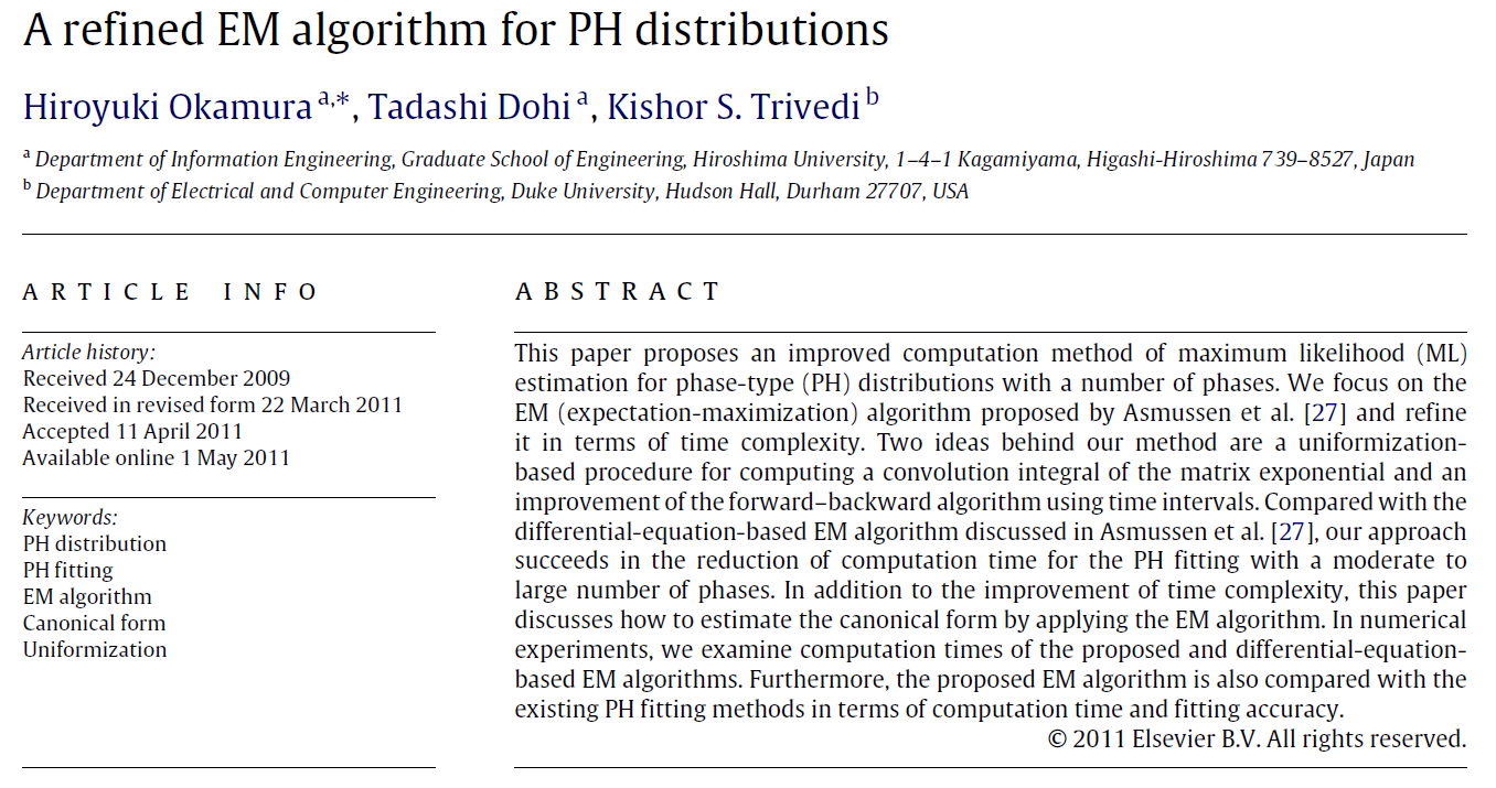
- If you really care about the details, check out our paper
- What are phase-type distributions? Why are they interesting?
- I have a package to fit them in the Julia language.
If you've never tried Julia, go for it.
\dagger
1
3
2
\overline{\boldsymbol{T}} = \left( \begin{matrix}
-6 & 4 & 2 & 0 \\
1 & -1 & 0 & 0 \\
0 & 5 & -5.5 & 0.5 \\
0 & 0 & 0 & 0
\end{matrix} \right)
\boldsymbol{\alpha} = ( \frac13, \frac13, \frac13, 0 )^\top
2
4
1
0.5
5
What are phase-type distributions?
Markov chain State space
( X_t )_{t \ge 0}
\{1, ..., p, \dagger \}
Phase-type definition
Markov chain State space
- Initial distribution
- Sub-transition matrix
- Exit rates
\boldsymbol{\alpha}
\boldsymbol{T}
\boldsymbol{t} = -\boldsymbol{T} 1
\boldsymbol{t}
\tau = \inf_t \{ X_t = \dagger \}
( X_t )_{t \ge 0}
\{1, ..., p, \dagger \}
\Leftrightarrow \tau \sim \mathrm{PhaseType}(\boldsymbol{\alpha}, \boldsymbol{T})
\overline{\boldsymbol{T}} = \left( \begin{matrix}
\boldsymbol{T} & \boldsymbol{t} \\
0 & 0
\end{matrix} \right)
Two ways to view the phases
As meaningless mathematical artefacts
Choose number of phases to balance accuracy and over-fitting
As states which reflect some part of reality
Choose number of phases to match reality
X.S. Lin & X. Liu (2007) Markov aging process and phase-type law of mortality.
N. Amer. Act J. 11, pp. 92-109
M. Govorun, G. Latouche, & S. Loisel (2015). Phase-type aging modeling for health dependent costs. Insurance: Mathematics and Economics, 62, pp. 173-183.
Phase-type properties
Matrix exponential
Density and tail
Moments
Laplace transform
f_\tau(s) = \boldsymbol{\alpha}^\top \mathrm{e}^{\boldsymbol{T} s} \boldsymbol{t}
\mathrm{e}^{\boldsymbol{T} s} = \sum_{i=0}^\infty \frac{(\boldsymbol{T} s)^i}{i!}
\tau \sim \mathrm{PhaseType}(\boldsymbol{\alpha}, \boldsymbol{T})
\overline{F}_\tau(s) = \boldsymbol{\alpha}^\top \mathrm{e}^{\boldsymbol{T} s} 1
\mathbb{E}[\tau] = {-}\boldsymbol{\alpha}^\top \boldsymbol{T}^{-1} \boldsymbol{1}
\mathbb{E}[\tau^n] = (-1)^n n! \,\, \boldsymbol{\alpha}^\top \boldsymbol{T}^{-n} \boldsymbol{1}
\mathbb{E}[\mathrm{e}^{-s\tau}] = \boldsymbol{\alpha}^\top (s \boldsymbol{I} - \boldsymbol{T})^{-1} \boldsymbol{t}
Class of phase-types is dense
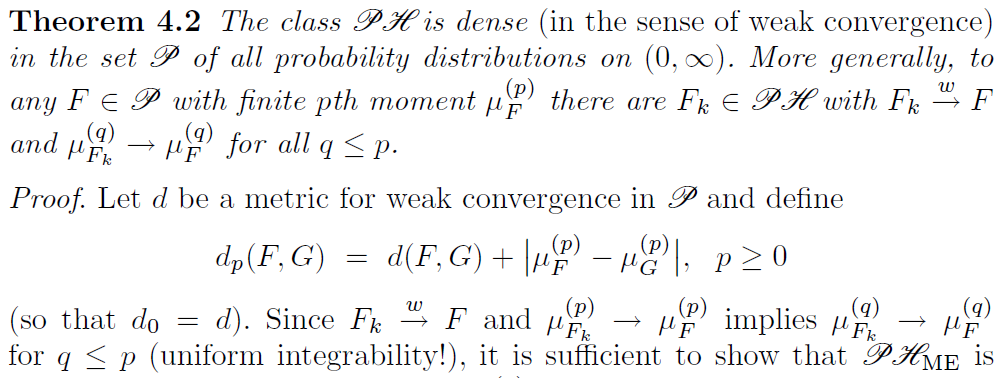
S. Asmussen (2003), Applied Probability and Queues, 2nd Edition, Springer
Phase-type generalises...
- Exponential distribution
- Sums of exponentials (Erlang distribution)
- Mixtures of exponentials (hyperexponential distribution)
\boldsymbol{\alpha} = \left( 1 \right), \boldsymbol{T} = \left( -\lambda \right), \boldsymbol{t} = \left( \lambda \right)
\boldsymbol{\alpha} = \left( \begin{matrix}
1 \\
0 \\
0
\end{matrix} \right) ,
\boldsymbol{T} = \left( \begin{matrix}
-\lambda_1 & \lambda_1 & 0 \\
0 & -\lambda_2 & \lambda_2 \\
0 & 0 & -\lambda_3
\end{matrix} \right)
, \boldsymbol{t} = \left( \begin{matrix}
0 \\
0 \\
\lambda_3
\end{matrix} \right)
\boldsymbol{\alpha} = \left( \begin{matrix}
\alpha_1 \\
\alpha_2 \\
\alpha_3
\end{matrix} \right) ,
\boldsymbol{T} = \left( \begin{matrix}
-\lambda_1 & 0 & 0 \\
0 & -\lambda_2 & 0 \\
0 & 0 & -\lambda_3
\end{matrix} \right)
, \boldsymbol{t} =
\left( \begin{matrix}
\lambda_1 \\
\lambda_2 \\
\lambda_3
\end{matrix} \right)
More cool properties
Closure under addition, minimum, maximum
(\tau \mid \tau > s) \sim \mathrm{PhaseType}(\boldsymbol{\alpha}_s, \boldsymbol{T})
\tau_i \sim \mathrm{PhaseType}(\boldsymbol{\alpha}_i, \boldsymbol{T}_i)
\Rightarrow \tau_1 + \tau_2 \sim \mathrm{PhaseType}(\dots, \dots)
\Rightarrow \min\{ \tau_1 , \tau_2 \} \sim \mathrm{PhaseType}(\dots, \dots)
... and under conditioning
\tau_n \sim \mathrm{Erlang}(n, n/T) \,, \quad \tau_n \approx T
Can make a phase-type look like a constant value
Contract over a limited horizon
\begin{aligned}
\tau \wedge T &\approx \tau \wedge \tau_n \\
&= \tau_n^* \sim \mathrm{PhaseType}(\dots, \dots)
\end{aligned}
\text{Price} \approx \mathbb{E}[ \mathrm{e}^{-\delta \tau_n^* } \text{Payoff}( S_{\tau_n^*}, \overline{S}_{\tau_n^*} ) ]
Payout occurs at death or after fixed duration T, whichever first
\text{Price} = \mathbb{E}[ \mathrm{e}^{-\delta (\tau \wedge T)} \text{Payoff}( S_{\tau \wedge T}, \overline{S}_{\tau \wedge T} ) ]
If it works for exponential distribution, try phase-type
Assume:
- is exponentially distributed
- where is a Brownian motion
Then and are independent and exponentially distributed with rates
\tau
S_t = \mathrm{e}^{X_t}
X_t
\overline{X}_\tau
\overline{X}_\tau - X_\tau
\lambda_{\pm} = \mp \frac{\mu}{\sigma^2} + \sqrt{ \frac{\mu^2}{\sigma^4} + \frac{2\lambda}{\sigma^2} }
\lambda
\mu, \sigma^2
Wiener-Hopf Factorisation
\mathbb{P}(\overline{X}_\tau \in \mathrm{d}x, X_\tau - \overline{X}_\tau \in \mathrm{d}y) = \mathbb{P}(\overline{X}_\tau \in \mathrm{d}x) \mathbb{P}(\underline{X}_\tau \in \mathrm{d}y)
X_t
-
is an exponential random variable
- is a Lévy process
\tau
Doesn't work for non-random time
\mathbb{P}(\overline{X}_t \in \mathrm{d}x, X_t - \overline{X}_t \in \mathrm{d}y \mid \overline{\sigma}_t = s)
= \mathbb{P}(\overline{X}_t \in \mathrm{d}x \mid \overline{\sigma}_t = s) \mathbb{P}(\underline{X}_t \in \mathrm{d}y \mid \underline{\sigma}_t = t - s)
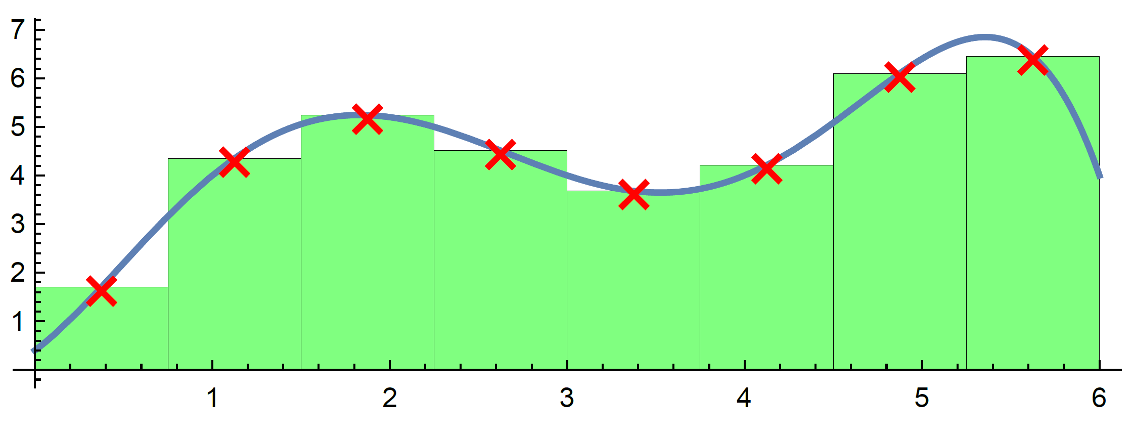
How to fit them?
Traditionally, using EM algorithm
Bladt, M., Gonzalez, A. and Lauritzen, S. L. (2003), ‘The estimation of Phase-type related functionals using Markov chain Monte Carlo methods’, Scandinavian Actuarial Journal

Representation is not unique
\boldsymbol{\alpha} = ( 1, 0, 0 )^\top
\boldsymbol{T}_1 = \left( \begin{matrix}
-1 & 1 & 0 \\
0 & -2 & 2 \\
0 & 0 & -3
\end{matrix} \right)
\boldsymbol{T}_2 = \left( \begin{matrix}
-3 & 3 & 0 \\
0 & -2 & 2 \\
0 & 0 & -1
\end{matrix} \right)
\tau_1 \sim \mathrm{PhaseType}(\boldsymbol{\alpha}, \boldsymbol{T}_1)
\tau_2 \sim \mathrm{PhaseType}(\boldsymbol{\alpha}, \boldsymbol{T}_2)
\tau_1 \overset{\mathscr{D}}{=} \tau_2
Also, not easy to tell if any parameters produce a valid distribution
Lots of parameters to fit
- General
- Coxian distribution
\boldsymbol{\alpha} = \left( \begin{matrix}
1 \\
0 \\
0
\end{matrix} \right) , \quad
\boldsymbol{T} = \left( \begin{matrix}
-\lambda_1 & \lambda_{12} & 0 \\
0 & -\lambda_2 & \lambda_{23} \\
0 & 0 & -\lambda_3
\end{matrix} \right)
\boldsymbol{\alpha} = \left( \begin{matrix}
\alpha_1 \\
\alpha_2 \\
\alpha_3
\end{matrix} \right) , \quad
\boldsymbol{T} = \left( \begin{matrix}
-\lambda_1 & \lambda_{12} & \lambda_{13} \\
\lambda_{21} & -\lambda_2 & \lambda_{23} \\
\lambda_{31} & \lambda_{32} & -\lambda_3
\end{matrix} \right)
p(p+1)-1
2p-1
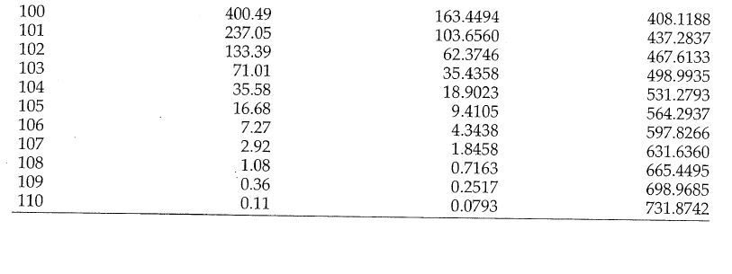
Problem: to model mortality via phase-type
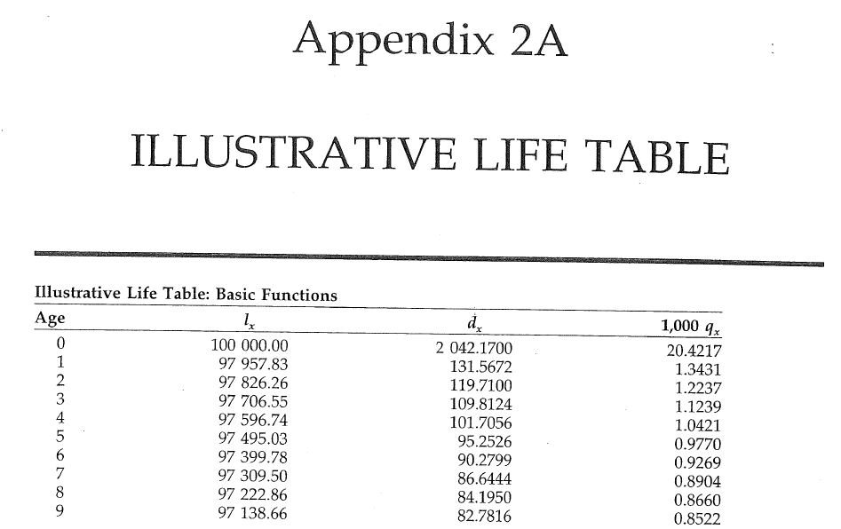
Bowers et al (1997), Actuarial Mathematics, 2nd Edition
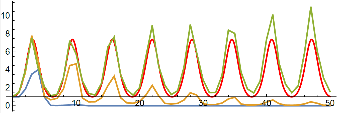
Fit General Phase-type with C

p = 5
p = 10
p = 20
\text{Life Table}
Why's this so terrible?
\mathrm{e}^{\boldsymbol{T} s} = \sum_{i=0}^\infty \frac{(\boldsymbol{T} s)^i}{i!}
"E" step has a bazillion matrix exponential calculations
Fit Coxian distributions
p = 5
p = 10
p = 20
\text{Life Table}
General vs Coxian
Rewrite in Julia
void rungekutta(int p, double *avector, double *gvector, double *bvector,
		double **cmatrix, double dt, double h, double **T, double *t,
		double **ka, double **kg, double **kb, double ***kc)
{
  int i, j, k, m;
  double eps, h2, sum;

  i = dt/h;
  h2 = dt/(i+1);
  init_matrix(ka, 4, p);
  init_matrix(kb, 4, p);
  init_3dimmatrix(kc, 4, p, p);
  if (kg != NULL)
    init_matrix(kg, 4, p);
    ...
    for (i=0; i < p; i++) {
      avector[i] += (ka[0][i]+2*ka[1][i]+2*ka[2][i]+ka[3][i])/6;
      bvector[i] += (kb[0][i]+2*kb[1][i]+2*kb[2][i]+kb[3][i])/6;
      for (j=0; j < p; j++)
        cmatrix[i][j] +=(kc[0][i][j]+2*kc[1][i][j]+2*kc[2][i][j]+kc[3][i][j])/6;
    }
  }
}
This function: 116 lines of C, built-in to Julia
Whole program: 1700 lines of C, 300 lines of Julia
# Run the ODE solver.
u0 = zeros(p*p)
pf = ParameterizedFunction(ode_observations!, fit)
prob = ODEProblem(pf, u0, (0.0, maximum(s.obs)))
sol = solve(prob, OwrenZen5())
https://github.com/Pat-Laub/EMpht.jl
DE solver going negative
# Run the ODE solver.
u0 = zeros(p*p)
pf = ParameterizedFunction(ode_observations!, fit)
prob = ODEProblem(pf, u0, (0.0, maximum(s.obs)))
sol = solve(prob, OwrenZen5())

...

u = sol(s.obs[k])
C = reshape(u, p, p)
if minimum(C) < 0
    (C,err) = hquadrature(p*p, (x,v) -> c_integrand(x, v, fit, s.obs[k]),
                0, s.obs[k], reltol=1e-1, maxevals=500)
    C = reshape(C, p, p)
end
Swap to quadrature in Julia
Fit Coxian with more phases

p = 50
p = 75
p = 100
\text{Life Table}
Coxian: Small p vs Big p
Uniformization magic
Coxian with uniformization

p = 50
p = 75
p = 100
\text{Life Table}
ODE vs Uniformization
A twist on the Coxian form
Canonical form 1
\boldsymbol{\alpha} = \left( \begin{matrix}
\alpha_1 \\
\alpha_2 \\
\alpha_3
\end{matrix} \right) , \quad
\boldsymbol{T} = \left( \begin{matrix}
-\lambda_1 & \lambda_1 & 0 \\
0 & -\lambda_2 & \lambda_2 \\
0 & 0 & -\lambda_3
\end{matrix} \right)
\lambda_1 < \lambda_2 < \dots < \lambda_p
Et voilà

p = 200
\text{Life Table}
using Pkg; Pkg.add("EMpht")

using EMpht
lt = EMpht.parse_settings("life_table.json")[1]

phCF200 = empht(lt, p=200, ph_structure="CanonicalForm1")
Julia Package Published


Remember to try Julia
Thanks for listening!
IME Talk
By plaub


