Phase-Type Models in
Life Insurance

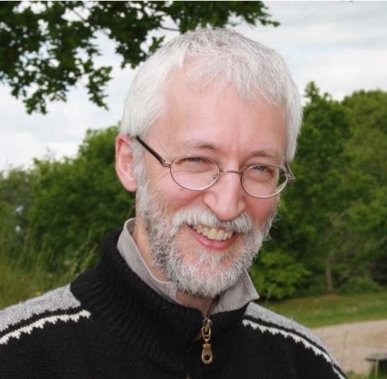
Dr Patrick J. Laub

Who am I?

Software Engineering and Mathematics
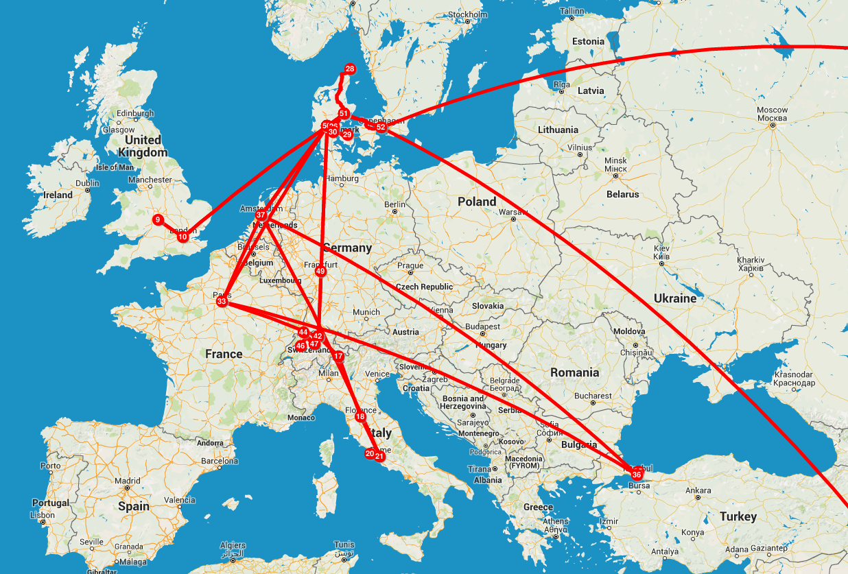
PhD between University of Queensland (Brisbane) and Aarhus University
PhD supervisors:
- Søren Asmussen
- Phil Pollett

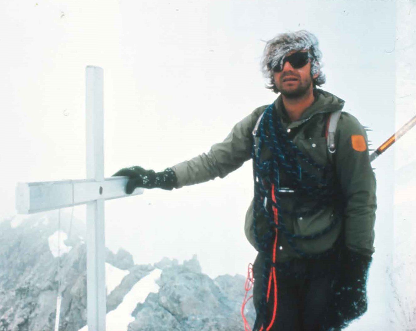
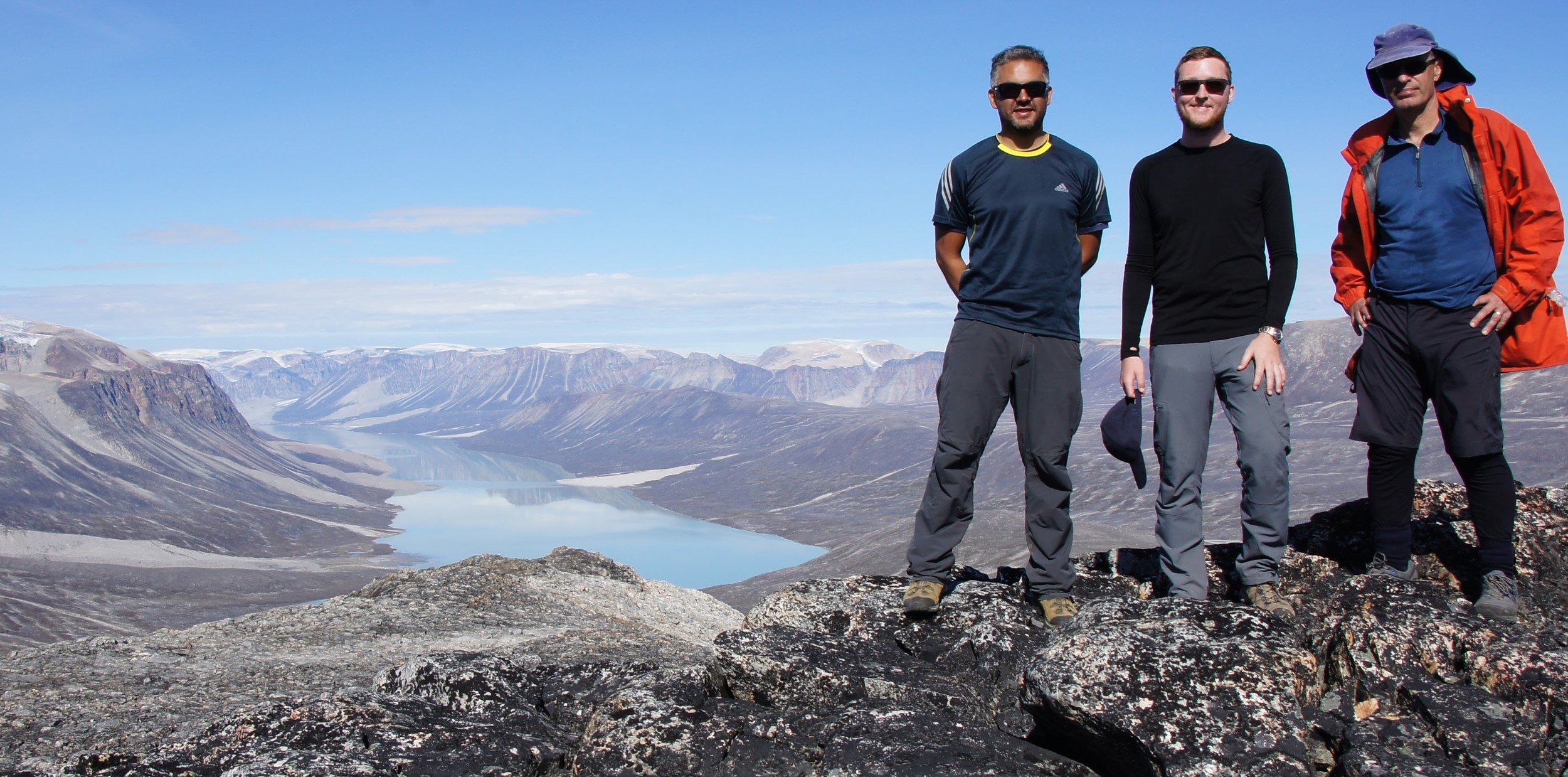
C'est moi!

Computational methods for sums of random variables

Mackay

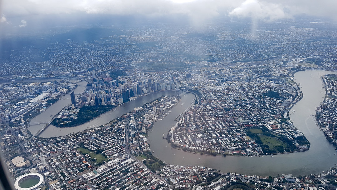
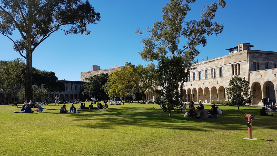
Brisbane (University of Queensland)

Software experience

Assembly
Bash
C
C#
C++
CSS
Dart
HTML
Java
JavaScript
Jekyll (Markdown)

Julia
LaTeX
Mathematica
Matlab
Perl
PHP
Python
R
Ruby (on Rails)
SQL
Visual Basic

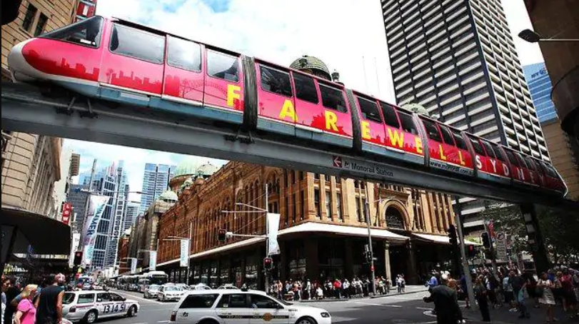
Sydney

Masters: Hawkes Processes

Paper version of my thesis on https://arxiv.org/abs/1507.02822

Monte Carlo

\pi \approx \, ?

Cross-entropy example

\mathbb{P}(Z > 5) \approx ? \qquad Z \sim \mathcal{N}(0,1)

Cross-entropy example

\mathbb{P}(\frac{1}{10} \int_0^{10} B(\mathrm{d} t) \ge 10) \approx \, ?

PhD outline

2015	Aarhus
2016 Jan-Jul	Brisbane
2016 Aug-Dec	Aarhus
2017	Brisbane/Melbourne
2018 Jan-Apr (end)	China

Supervisors: Søren Asmussen, Phil Pollett, and Jens L. Jensen

Laplace transform approximation for sums of dependent lognormals

\mathscr{L}_X(t) = \overline{\mathscr{L}}_X(t) (1 + \mathcal{O}(\frac{1}{\log(t)}))

No closed-form exists for a single lognormal

Asmussen, S., Jensen, J. L., & Rojas-Nandayapa, L. (2016). On the Laplace transform of the lognormal distribution. Methodology and Computing in Applied Probability

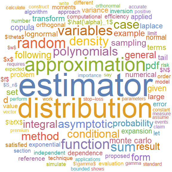
Orthogonal polynomial expansions

Choose a reference distribution, e.g,

\nu = \mathsf{Gamma}(r,m) \Rightarrow f_\nu(x) \propto x^{r-1}\mathrm{e}^{-\frac{x}{m}}

2. Find its orthogonal polynomial system

\{ Q_n(x) \}_{n\in \mathbb{N}_0}

f_X(x) = f_\nu(x) \times \sum_{k=0}^\infty q_k Q_k(x)

3. Construct the polynomial expansion

Pierre-Olivier Goffard

Asmussen, S., Goffard, P. O., & Laub, P. J. (2017). Orthonormal polynomial expansions and lognormal sum densities. Risk and Stochastics - Festschrift for Ragnar Norberg (to appear).

My Thesis

Søren visits Melbourne

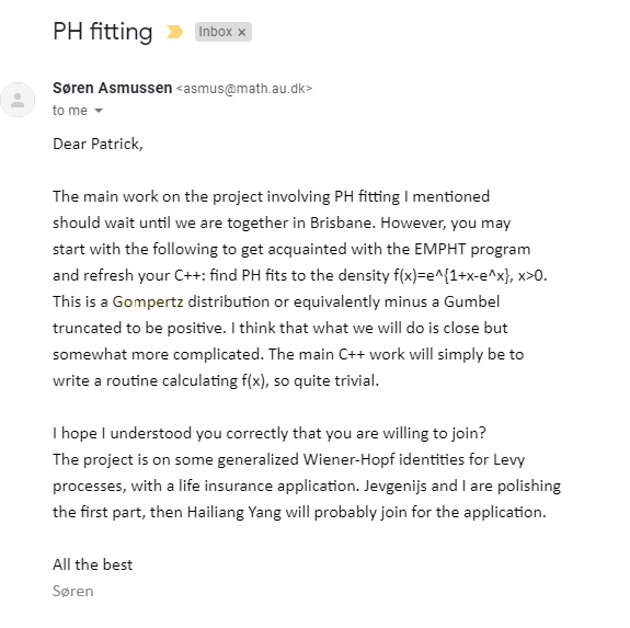
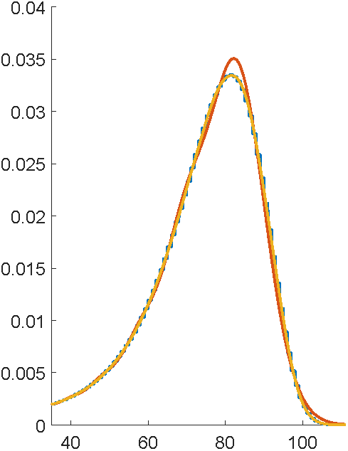
Problem: to model mortality via phase-type

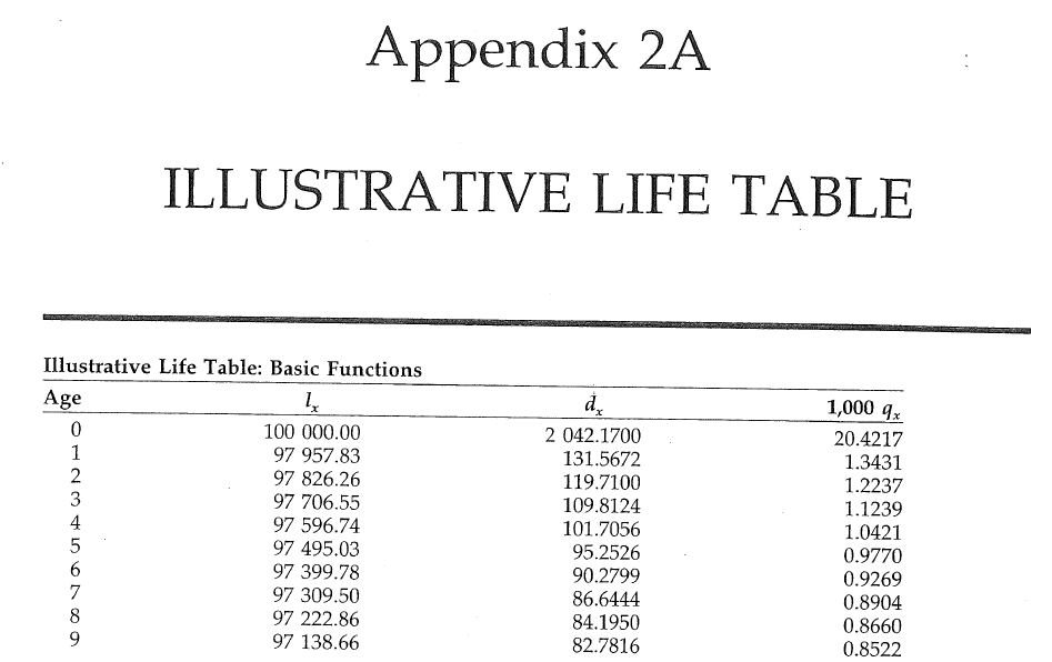
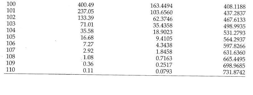
Bowers et al (1997), Actuarial Mathematics, 2nd Edition

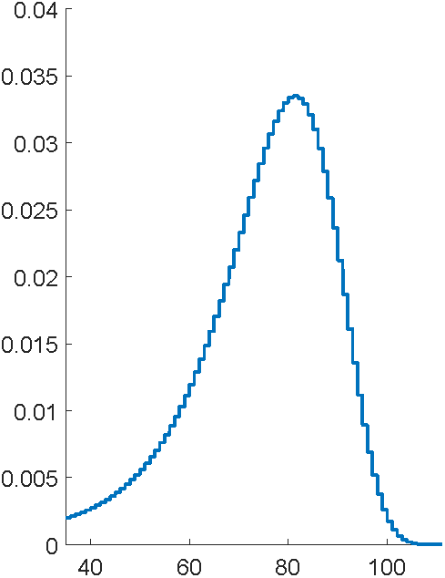
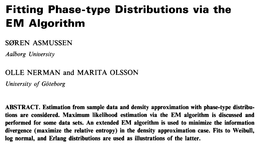
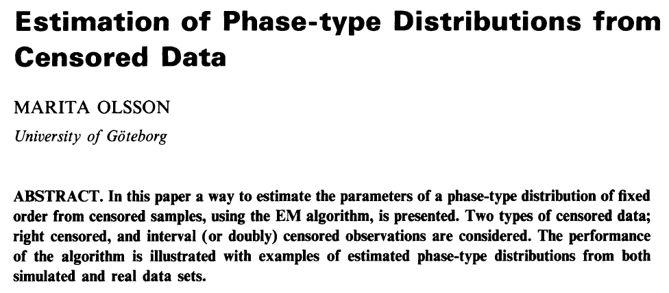
... using the C code EMpht

\dagger

1

3

2

\overline{T} = \left( \begin{matrix} -6 & 4 & 2 & 0 \\ 1 & -1 & 0 & 0 \\ 0 & 5 & -5.5 & 0.5 \\ 0 & 0 & 0 & 0 \end{matrix} \right)

\alpha = ( \frac13, \frac13, \frac13, 0 )^\top

2

4

1

0.5

5

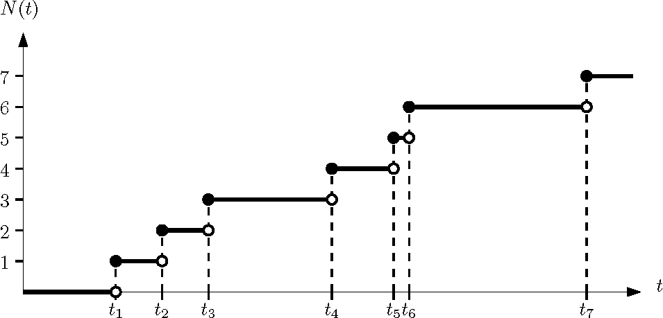
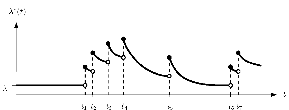
What are phase-type distributions?

Markov chain State space

( X_t )_{t \ge 0}

\{1, ..., p, \dagger \}

Phase-type distributions

Markov chain State space

( X_t )_{t \ge 0}

\{1, ..., p, \dagger \}

Phase-type definition

Markov chain State space

Initial distribution
Sub-transition matrix
Exit rates

\alpha

T

t = -T 1

t

\tau = \inf_t \{ X_t = \dagger \}

( X_t )_{t \ge 0}

\{1, ..., p, \dagger \}

\Leftrightarrow \tau \sim \mathrm{PhaseType}(\alpha, T)

\overline{T} = \left( \begin{matrix} T & t \\ 0 & 0 \end{matrix} \right)

Phase-type properties

Matrix exponential

Density and tail

Moments

M.g.f

f_\tau(s) = \alpha^\top \mathrm{e}^{T s} t

\mathrm{e}^{T s} = \sum_{i=0}^\infty \frac{(T s)^i}{i!}

\tau \sim \mathrm{PhaseType}(\alpha, T)

\overline{F}_\tau(s) = \alpha^\top \mathrm{e}^{T s} 1

\mathbb{E}[\tau] = {-}\alpha^\top T^{-1} 1

\mathbb{E}[\tau^n] = (-1)^n n! \,\, \alpha^\top T^{-n} 1

Phase-type generalises...

Exponential distribution
Sums of exponentials (Erlang distribution)
Mixtures of exponentials (hyperexponential distribution)

\alpha = \left( 1 \right), T = \left( -\lambda \right), t = \left( \lambda \right)

\alpha = \left( \begin{matrix} 1 \\ 0 \\ 0 \end{matrix} \right) , T = \left( \begin{matrix} -\lambda_1 & \lambda_1 & 0 \\ 0 & -\lambda_2 & \lambda_2 \\ 0 & 0 & -\lambda_3 \end{matrix} \right) , t = \left( \begin{matrix} 0 \\ 0 \\ \lambda_3 \end{matrix} \right)

\alpha = \left( \begin{matrix} \alpha_1 \\ \alpha_2 \\ \alpha_3 \end{matrix} \right) , T = \left( \begin{matrix} -\lambda_1 & 0 & 0 \\ 0 & -\lambda_2 & 0 \\ 0 & 0 & -\lambda_3 \end{matrix} \right) , t = \left( \begin{matrix} \lambda_1 \\ \lambda_2 \\ \lambda_3 \end{matrix} \right)

Class of phase-types is dense

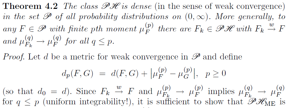
S. Asmussen (2003), Applied Probability and Queues, 2nd Edition, Springer

More cool properties

Closure under addition, minimum, maximum

(\tau \mid \tau > s) \sim \mathrm{PhaseType}(\alpha_s, T)

\tau_i \sim \mathrm{PhaseType}(\alpha_i, T_i)

\Rightarrow \tau_1 + \tau_2 \sim \mathrm{PhaseType}(\dots, \dots)

\Rightarrow \min\{ \tau_1 , \tau_2 \} \sim \mathrm{PhaseType}(\dots, \dots)

\alpha_s^\top = \overline{F}_\tau(s)^{-1} \alpha^\top \mathrm{e}^{T s}

... and under conditioning

Erlangization/Canadization

T \in \mathbb{R} \qquad \tau_n \sim \mathrm{Erlang}(n, n/T)

\tau_n \overset{\mathbb{P}}{\longrightarrow} T \qquad \text{as } n \to \infty

Phase-type can even approximate a constant!

Representation is not unique

\alpha = ( 1, 0, 0 )^\top

T_1 = \left( \begin{matrix} -1 & 1 & 0 \\ 0 & -2 & 2 \\ 0 & 0 & -3 \end{matrix} \right)

T_2 = \left( \begin{matrix} -3 & 3 & 0 \\ 0 & -2 & 2 \\ 0 & 0 & -1 \end{matrix} \right)

\tau_1 \sim \mathrm{PhaseType}(\alpha, T_1)

\tau_2 \sim \mathrm{PhaseType}(\alpha, T_2)

\tau_1 \overset{\mathscr{D}}{=} \tau_2

Also, not easy to tell if any parameters produce a valid distribution

Lots of parameters to fit

General
Coxian distribution
Generalised Coxian distribution

\alpha = \left( \begin{matrix} 1 \\ 0 \\ 0 \end{matrix} \right) , \quad T = \left( \begin{matrix} -\lambda_1 & \lambda_{12} & 0 \\ 0 & -\lambda_2 & \lambda_{23} \\ 0 & 0 & -\lambda_3 \end{matrix} \right)

\alpha = \left( \begin{matrix} \alpha_1 \\ \alpha_2 \\ \alpha_3 \end{matrix} \right) , \quad T = \left( \begin{matrix} -\lambda_1 & \lambda_{12} & 0 \\ 0 & -\lambda_2 & \lambda_{23} \\ 0 & 0 & -\lambda_3 \end{matrix} \right)

\alpha = \left( \begin{matrix} \alpha_1 \\ \alpha_2 \\ \alpha_3 \end{matrix} \right) , \quad T = \left( \begin{matrix} -\lambda_1 & \lambda_{12} & \lambda_{13} \\ \lambda_{21} & -\lambda_2 & \lambda_{23} \\ \lambda_{31} & \lambda_{32} & -\lambda_3 \end{matrix} \right)

p(p+1)-1

2p-1

3p-2

Generalised Coxian

Two ways to view the phases

As meaningless mathematical artefacts

Choose number of phases to balance accuracy and over-fitting

As states which reflect some part of reality

Choose number of phases to match reality

X.S. Lin & X. Liu (2007) Markov aging process and phase-type law of mortality.
N. Amer. Act J. 11, pp. 92-109

M. Govorun, G. Latouche, & S. Loisel (2015). Phase-type aging modeling for health dependent costs. Insurance: Mathematics and Economics, 62, pp. 173-183.

Valuing equity-linked life insurance products

Say the customer lives for years
Payout at death is linked to equity
Example:
- Guaranteed Minimum Death Benefit
- High Water Benefit
Need

\tau

S_t

\max( S_{\tau}, K )

\overline{S}_\tau = \max_{t \le \tau} S_t

\mathbb{E}[ \mathrm{e}^{-\delta \tau} \Psi(\overline{S}_\tau, S_\tau) ]

Simplest model

Assume:

is exponentially distributed
where is a Brownian motion

Then and are independent and exponentially distributed with rates

\tau

S_t = \mathrm{e}^{X_t}

X_t

\overline{X}_\tau

\overline{X}_\tau - X_\tau

\lambda_{\pm} = \mp \frac{\mu}{\sigma^2} + \sqrt{ \frac{\mu^2}{\sigma^4} + \frac{2\lambda}{\sigma^2} }

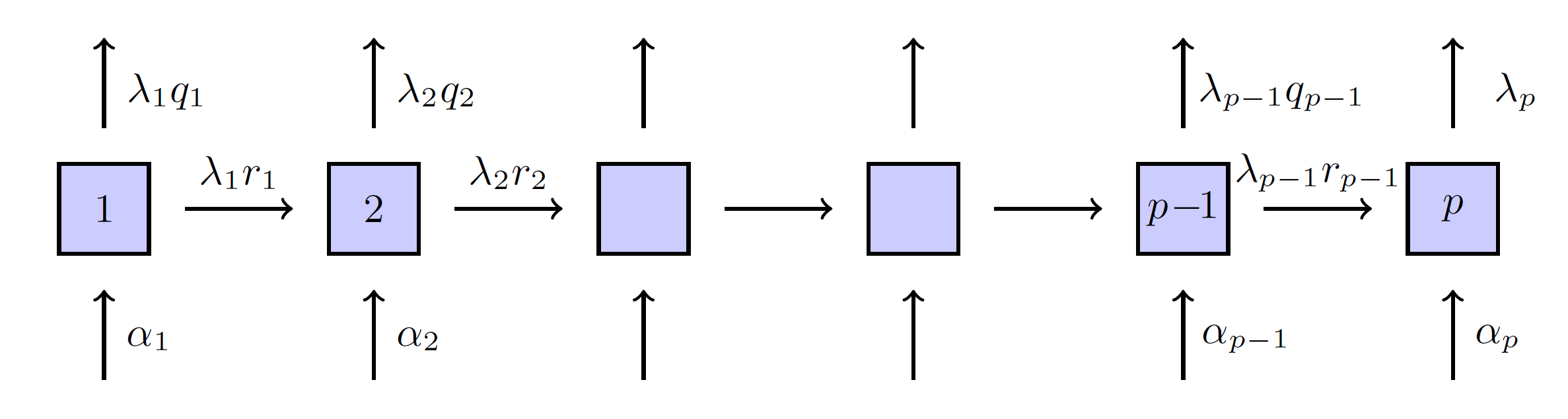
Wiener-Hopf Factorisation

\mathbb{P}(\overline{X}_\tau \in \mathrm{d}x, X_\tau - \overline{X}_\tau \in \mathrm{d}y) = \mathbb{P}(\overline{X}_\tau \in \mathrm{d}x) \mathbb{P}(\underline{X}_\tau \in \mathrm{d}y)

X_t

is an exponential random variable
is a Lévy process

\tau

Doesn't work for non-random time

\mathbb{P}(\overline{X}_t \in \mathrm{d}x, X_t - \overline{X}_t \in \mathrm{d}y \mid \overline{\sigma}_t = s)

= \mathbb{P}(\overline{X}_t \in \mathrm{d}x \mid \overline{\sigma}_t = s) \mathbb{P}(\underline{X}_t \in \mathrm{d}y \mid \underline{\sigma}_t = t - s)

Motivating theory

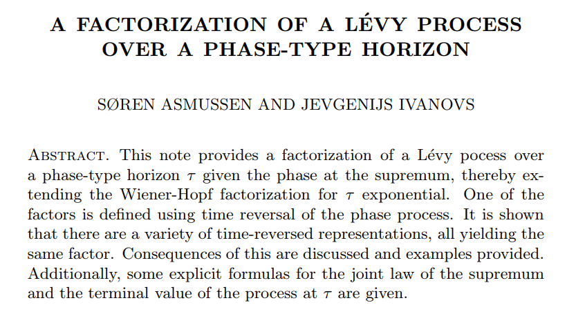
Accepted to Stochastic Models

Can read on https://arxiv.org/pdf/1803.00273.pdf

First attempts with EMpht

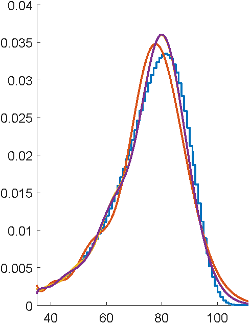
5 hours compute time

This is ancient technology...

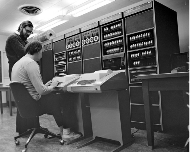
Dennis Ritchie (creator of C) standing by the computer used to create C, 1972

Diving into the source

c(y ; i \mid \alpha, T) = \int_0^y \alpha^\top \mathrm{e}^{T u} e_i \cdot \mathrm{e}^{T (y-u)} t \,\, \mathrm{d} u

i = 1, \dots, p

Single threaded
Homegrown matrix handling (e.g. all dense)
Computational "E" step
Instead solve a large system of DEs
Hard to read or modify (e.g. random function)

c'(y ; i \mid \alpha, T) = T c(y ; i \mid \alpha, T) + [ \alpha^ \top \mathrm{e}^{T y} ]_i t

p(p+2)

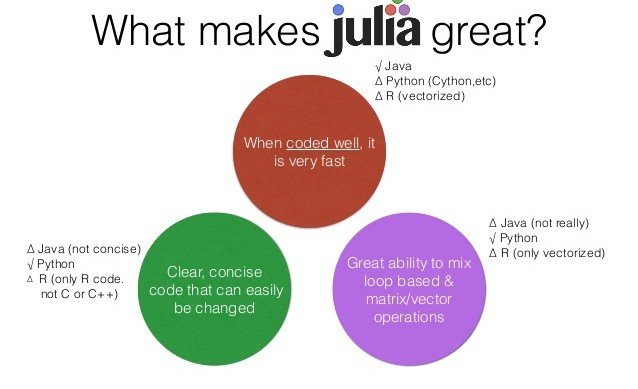
Rewrite in Julia

void rungekutta(int p, double *avector, double *gvector, double *bvector,
		double **cmatrix, double dt, double h, double **T, double *t,
		double **ka, double **kg, double **kb, double ***kc)
{
  int i, j, k, m;
  double eps, h2, sum;

  i = dt/h;
  h2 = dt/(i+1);
  init_matrix(ka, 4, p);
  init_matrix(kb, 4, p);
  init_3dimmatrix(kc, 4, p, p);
  if (kg != NULL)
    init_matrix(kg, 4, p);
    ...
    for (i=0; i < p; i++) {
      avector[i] += (ka[0][i]+2*ka[1][i]+2*ka[2][i]+ka[3][i])/6;
      bvector[i] += (kb[0][i]+2*kb[1][i]+2*kb[2][i]+kb[3][i])/6;
      for (j=0; j < p; j++)
        cmatrix[i][j] +=(kc[0][i][j]+2*kc[1][i][j]+2*kc[2][i][j]+kc[3][i][j])/6;
    }
  }
}

This function: 116 lines of C, built-in to Julia

Whole program: 1700 lines of C, 300 lines of Julia

# Run the ODE solver.
u0 = zeros(p*p)
pf = ParameterizedFunction(ode_observations!, fit)
prob = ODEProblem(pf, u0, (0.0, maximum(s.obs)))
sol = solve(prob, OwrenZen5())

https://github.com/Pat-Laub/EMpht.jl

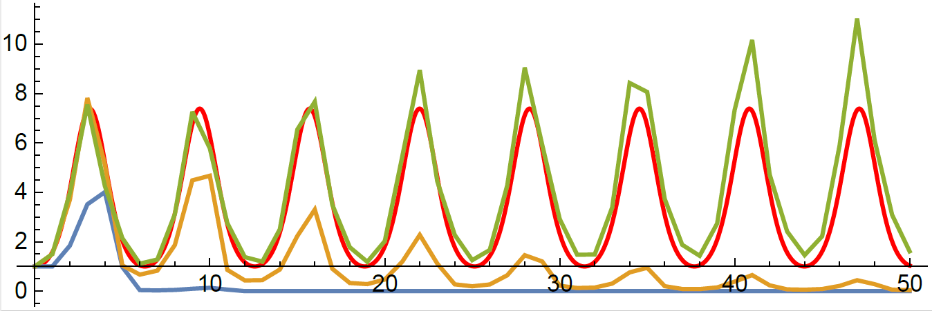
DE solver going negative

# Run the ODE solver.
u0 = zeros(p*p)
pf = ParameterizedFunction(ode_observations!, fit)
prob = ODEProblem(pf, u0, (0.0, maximum(s.obs)))
sol = solve(prob, OwrenZen5())

...

u = sol(s.obs[k])
C = reshape(u, p, p)
if minimum(C) < 0
    (C,err) = hquadrature(p*p, (x,v) -> c_integrand(x, v, fit, s.obs[k]), 
                0, s.obs[k], reltol=1e-1, maxevals=500)
    C = reshape(C, p, p)
end

Swap to quadrature in Julia

Rushing to complete

Submission deadline passes

Get to Lyon..

Uniformization magic

What was the point of all this again?

The customer lives for years
Need
... and we have it

where

\mathbb{E}[ \mathrm{e}^{-\delta \tau} \Psi(\overline{S}_\tau, S_\tau) ]

\tau

= \mathbb{E}[ \mathrm{e}^{-\delta \tau} \Psi( S_0 \mathrm{e}^{\overline{X}_\tau}, S_0 \mathrm{e}^{X_\tau} ) ]

\mathbb{E} [\mathrm{e}^{-\delta\tau} f(\overline{X}_\tau)g(D_\tau) ] = \alpha^\top F_{U_\delta} \Delta_r G_{U^*_\delta }^{\top}{\alpha^*}^{\!\top}

G_{U^*_\delta} = \int_0^\infty g(y)\mathrm{e}^{U^*_\delta y}\,\mathrm{d} y

F_{U_\delta} = \int_0^\infty f(x) \mathrm{e}^{U_\delta x}\,\mathrm{d} x \,,

Another cool thing

\mathbb{E}[ \mathrm{e}^{-\delta (\tau \wedge T) } \Psi(\overline{S}_{\tau \wedge T}, S_{\tau \wedge T}) ]

Contract over a limited horizon

Can use Erlangization so

\tau_n \approx T \,, \quad \tau_n \sim \mathrm{Erlang}(n, n/T)

\tau \wedge \tau_n = \tau_n^* \sim \mathrm{PhaseType}(\dots, \dots)

\ldots \approx \mathbb{E}[ \mathrm{e}^{-\delta \tau_n^* } \Psi(\overline{S}_{\tau_n^*}, S_{\tau_n^*}) ]

and phase-type closure under minimums

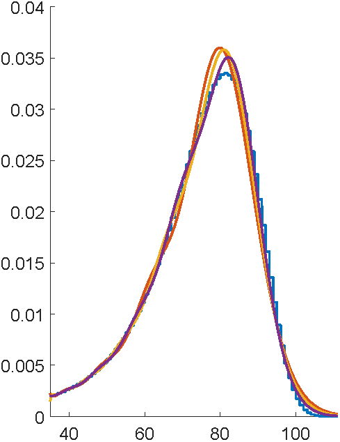
What conclusion to draw?

... [Phase-types] are not well suited to approximating every distribution. Despite the fact that they are dense... the order of the approximating distribution may be disappointingly large... while the phase-type distributions are admittedly poorly suited to matching certain features, even low-order phase-type distributions do display a great variety of shapes...This rich family may be used in place of exponential distributions in many models without destroying our ability to compute solutions.

C.A. O'Cinneide (1999), Phase-type distributions: open problems and a few properties, Stochastic Models 15(4), p. 4

Phase-Type Models in Life Insurance

Who am I?

Mackay

Brisbane (University of Queensland)

Software experience

Sydney

Masters: Hawkes Processes

Monte Carlo

Cross-entropy example

Cross-entropy example

PhD outline

Laplace transform approximation for sums of dependent lognormals

Orthogonal polynomial expansions

My Thesis

Søren visits Melbourne

Problem: to model mortality via phase-type

... using the C code EMpht

What are phase-type distributions?

Phase-type distributions

Phase-type definition

Phase-type properties

Phase-type generalises...

Class of phase-types is dense

More cool properties

Erlangization/Canadization

Representation is not unique

Lots of parameters to fit

Generalised Coxian

Two ways to view the phases

Valuing equity-linked life insurance products

Simplest model

Wiener-Hopf Factorisation

Motivating theory

First attempts with EMpht

This is ancient technology...

Diving into the source

Rewrite in Julia

DE solver going negative

Swap to quadrature in Julia

Swap to quadrature in Julia

Rushing to complete

Submission deadline passes

Get to Lyon..

Uniformization magic

Uniformization magic

What was the point of all this again?

Another cool thing

What conclusion to draw?

Phase-Type Models in Life Insurance

More from plaub

Phase-Type Models in
Life Insurance