Hypothesis

Testing

They are an American fast food chain that operates over 500 restaurants in the US and was started back in 1941. Today, they possess proprietary software called Smoke Stack which was built by service providers iOLAP. Smoke Stack reads data from POS systems, loyalty programs, promotions, surveys and inventory records and provides real-time feedback to improve sales and optimize other processes.

CIO Laura Rea Dickey believes Smoke Stack is the tool that gives them the competitive edge in the fast-paced casual food industry in the US. Decisions are taken based on insights provided by Smoke Stack every 20 minutes. A daily morning briefing at the corporate HQ enables higher level planning and execution of various strategies. A simple example of how Dickey’s make use of Smoke Stack – if data reveals that sales of chicken ribs have been low in a certain area and the store has a sizeable amount of ribs, text invitations are sent to customers in that area for ribs specials.

What if data suggest low sales while sale picks up later on - kind of False signal

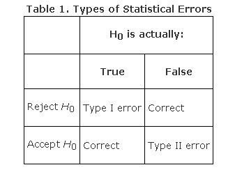
The initial belief is called the null hypothesis (H0)

Type I error is the incorrect rejection of a true null hypothesis

In other words, take action where none is required

Negation of Null Hypothesis is called the alternative hypothesis (H A , H a , H 1 )

Type II error is incorrectly retaining a false null hypothesis (also known as a "false negative" finding).

In other words, failing to take action where it is required

A Type I error is often represented by the Greek letter alpha (α) and a Type II error by the Greek letter beta (β ).

In choosing a level of probability for a test, you are actually deciding how much you want to risk committing a Type I error—rejecting the null hypothesis when it is, in fact, true.

For this reason, the area in the region of rejection is sometimes called the alpha level because it represents the likelihood of committing a Type I error.

Type I and Type II errors are inversely related: As one increases, the other decreases.

The Type I, or α (alpha), error rate is usually set in advance by the researcher.

The Type II error rate for a given test is harder to know because it requires estimating the distribution of the alternative hypothesis, which is usually unknown.

A related concept is power—the probability that a test will reject the null hypothesis when it is, in fact, false

High power is desirable. Like β, power can be difficult to estimate accurately, but increasing the sample size always increases power.

Problem 1

Suppose the manufacturer claims that the mean lifetime of a light bulb is more than 10,000 hours. In a sample of 30 light bulbs, it was found that they only last 9,900 hours on average. Assume the population standard deviation is 120 hours. At .05 significance level, can we reject the claim by the manufacturer?

Problem 1

Solution

The null hypothesis is that μ ≥ 10000. We begin with computing the test statistic.

xbar = 9900            # sample mean 
mu0 = 10000            # hypothesized value 
sigma = 120            # population standard deviation 
n = 30                 # sample size 
z = (xbar - mu0)/(sigma/sqrt(n))
z                      # test statistic

We then compute the critical value at .05 significance level.

alpha = .05 
z.alpha = qnorm(1-alpha) 
-z.alpha               # critical value

Answer

The test statistic -4.5644 is less than the critical value of -1.6449. Hence, at .05 significance level, we reject the claim that mean lifetime of a light bulb is above 10,000 hours.

Alternative Solution

Instead of using the critical value, we apply the pnorm function to compute the lower tail p-value of the test statistic. As it turns out to be less than the .05 significance level, we reject the null hypothesis that μ ≥ 10000.

pval = pnorm(z)
pval                   # lower tail p−value

When you perform a hypothesis test in statistics, a p-value helps you determine the significance of your results. ... The p-value is a number between 0 and 1 and interpreted in the following way: A small p-value (typically ≤ 0.05) indicates strong evidence against the null hypothesis, so you reject the null hypothesis.

Problem 2

Suppose the food label on a cookie bag states that there is at most 2 grams of saturated fat in a single cookie. In a sample of 35 cookies, it is found that the mean amount of saturated fat per cookie is 2.1 grams. Assume that the population standard deviation is 0.25 grams. At .05 significance level, can we reject the claim on food label?

Solution

The null hypothesis is that μ ≤ 2. We begin with computing the test statistic.

We then compute the critical value at .05 significance level.

xbar = 2.1             # sample mean
mu0 = 2                # hypothesized value
sigma = 0.25           # population standard deviation
n = 35                 # sample size
z = (xbar - mu0)/(sigma/sqrt(n))
z                      # test statistic

alpha = .05
z.alpha = qnorm(1−alpha)
z.alpha                # critical value

Answer

The test statistic 2.3664 is greater than the critical value of 1.6449. Hence, at .05 significance level, we reject the claim that there is at most 2 grams of saturated fat in a cookie.

Alternative Solution

Instead of using the critical value, we apply the pnorm function to compute the upper tail p-value of the test statistic. As it turns out to be less than the .05 significance level, we reject the null hypothesis that μ ≤ 2.

pval = pnorm(z, lower.tail=FALSE) 
pval

Problem 3

Suppose the mean weight of King Penguins found in an Antarctic colony last year was 15.4 kg. In a sample of 35 penguins same time this year in the same colony, the mean penguin weight is 14.6 kg. Assume the population standard deviation is 2.5 kg. At .05 significance level, can we reject the null hypothesis that the mean penguin weight does not differ from last year?

Solution

The null hypothesis is that μ = 15.4. We begin with computing the test statistic.

We then compute the critical values at .05 significance level.

xbar = 14.6            # sample mean 
mu0 = 15.4             # hypothesized value 
sigma = 2.5            # population standard deviation 
n = 35                 # sample size 
z = (xbar-mu0)/(sigma/sqrt(n)) 
z                      # test statistic

alpha = .05 
z.half.alpha = qnorm(1-alpha/2) 
c(-z.half.alpha, z.half.alpha)

Answer

The test statistic -1.8931 lies between the critical values -1.9600 and 1.9600. Hence, at .05 significance level, we do not reject the null hypothesis that the mean penguin weight does not differ from last year.

Alternative Solution

Instead of using the critical value, we apply the pnorm function to compute the two-tailed p-value of the test statistic. It doubles the lower tail p-value as the sample mean is less than the hypothesized value. Since it turns out to be greater than the .05 significance level, we do not reject the null hypothesis that μ = 15.4.

pval = 2 * pnorm(z)    # lower tail
pval                   # two−tailed p−value

How to adjust the interval estimate if the population standard deviation is not known?

We replace σ with our best guess (point estimate) s, which is the standard deviation of the sample

\sqrt(1/(n-1) * \sum\limits_{i=1}^n(xi-\overline X)^2)

\sqrt(1/(n-1) * \sum\limits_{i=1}^n(xi-\overline X)^2)

s =

\bar x - \mu

\bar x - \mu

s / \sqrt(n)

s / \sqrt(n)

t =

Calculate

T Statistic

If the underlying population is normally distributed, T is a random variable distributed according to a t‐distribution with n‐1 degrees of freedom (T n‐1 )

Research has shown that the t‐distribution is fairly robust to deviations of the population from the normal model

Student's t-distribution

(or simply t-distribution)

As n -> , tn -> N(0,1)

\infty

\infty

i.e. as the degrees of freedom increase, the t-distribution approaches the standard normal distribution

Confidence Interval for Mean with Unknown σ

\bar X - t * s/\sqrt(n) \le T \le \bar X + t * s/\sqrt(n)

\bar X - t * s/\sqrt(n) \le T \le \bar X + t * s/\sqrt(n)

n-1

1- ,n-1

\alpha

\alpha

\alpha

\alpha

Problem

Suppose the manufacturer claims that the mean lifetime of a light bulb is more than 10,000 hours. In a sample of 30 light bulbs, it was found that they only last 9,900 hours on average. Assume the sample standard deviation is 125 hours. At .05 significance level, can we reject the claim by the manufacturer?

Solution

The null hypothesis is that μ ≥ 10000. We begin with computing the test statistic.

We then compute the critical value at .05 significance level.

> xbar = 9900            # sample mean 
> mu0 = 10000            # hypothesized value 
> s = 125                # sample standard deviation 
> n = 30                 # sample size 
> t = (xbar−mu0)/(s/sqrt(n)) 
> t                      # test statistic

> alpha = .05 
> t.alpha = qt(1−alpha, df=n−1) 
> -t.alpha               # critical value

Answer

The test statistic -4.3818 is less than the critical value of -1.6991. Hence, at .05 significance level, we can reject the claim that mean lifetime of a light bulb is above 10,000 hours.

Alternative Solution

Instead of using the critical value, we apply the pt function to compute the lower tail p-value of the test statistic. As it turns out to be less than the .05 significance level, we reject the null hypothesis that μ ≥ 10000.

> pval = pt(t, df=n−1) 
> pval                   # lower tail p−value

Problem

Suppose the food label on a cookie bag states that there is at most 2 grams of saturated fat in a single cookie. In a sample of 35 cookies, it is found that the mean amount of saturated fat per cookie is 2.1 grams. Assume that the sample standard deviation is 0.3 gram. At .05 significance level, can we reject the claim on food label?

Solution

The null hypothesis is that μ ≤ 2. We begin with computing the test statistic.

We then compute the critical value at .05 significance level.

> xbar = 2.1             # sample mean 
> mu0 = 2                # hypothesized value 
> s = 0.3                # sample standard deviation 
> n = 35                 # sample size 
> t = (xbar−mu0)/(s/sqrt(n)) 
> t                      # test statistic

> alpha = .05 
> t.alpha = qt(1−alpha, df=n−1) 
> t.alpha                # critical value

> pval = pt(t, df=n−1, lower.tail=FALSE) 
> pval                   # upper tail p−value

Answer

The test statistic 1.9720 is greater than the critical value of 1.6991. Hence, at .05 significance level, we can reject the claim that there is at most 2 grams of saturated fat in a cookie.

Alternative Solution

Instead of using the critical value, we apply the pt function to compute the upper tail p-value of the test statistic. As it turns out to be less than the .05 significance level, we reject the null hypothesis that μ ≤ 2.

Problem

Suppose the mean weight of King Penguins found in an Antarctic colony last year was 15.4 kg. In a sample of 35 penguins same time this year in the same colony, the mean penguin weight is 14.6 kg. Assume the sample standard deviation is 2.5 kg. At .05 significance level, can we reject the null hypothesis that the mean penguin weight does not differ from last year?

Solution

The null hypothesis is that μ = 15.4. We begin with computing the test statistic.

We then compute the critical values at .05 significance level.

> xbar = 14.6            # sample mean 
> mu0 = 15.4             # hypothesized value 
> s = 2.5                # sample standard deviation 
> n = 35                 # sample size 
> t = (xbar−mu0)/(s/sqrt(n)) 
> t                      # test statistic

> alpha = .05 
> t.half.alpha = qt(1−alpha/2, df=n−1) 
> c(−t.half.alpha, t.half.alpha)

Answer

The test statistic -1.8931 lies between the critical values -2.0322, and 2.0322. Hence, at .05 significance level, we do not reject the null hypothesis that the mean penguin weight does not differ from last year.

Alternative Solution

Instead of using the critical value, we apply the pt function to compute the two-tailed p-value of the test statistic. It doubles the lower tail p-value as the sample mean is less than the hypothesized value. Since it turns out to be greater than the .05 significance level, we do not reject the null hypothesis that μ = 15.4.

> pval = 2 ∗ pt(t, df=n−1)  # lower tail 
> pval                      # two−tailed p−value

Problem

Suppose the manufacturer claims that the mean lifetime of a light bulb is more than 10,000 hours. In a sample of 30 light bulbs, it was found that they only last 9,900 hours on average. Assume the sample standard deviation is 125 hours. At .05 significance level, can we reject the claim by the manufacturer?

Solution

The null hypothesis is that μ ≥ 10000. We begin with computing the test statistic.

We then compute the critical value at .05 significance level.

xbar = 9900            # sample mean 
mu0 = 10000            # hypothesized value 
s = 125                # sample standard deviation 
n = 30                 # sample size 
t = (xbar−mu0)/(s/sqrt(n)) 
t                      # test statistic

alpha = .05 
t.alpha = qt(1−alpha, df=n−1) 
−t.alpha               # critical value

Answer

The test statistic -4.3818 is less than the critical value of -1.6991. Hence, at .05 significance level, we can reject the claim that mean lifetime of a light bulb is above 10,000 hours.

Alternative Solution

pval = pt(t, df=n−1) 
pval                   # lower tail p−value

Problem

Suppose the food label on a cookie bag states that there is at most 2 grams of saturated fat in a single cookie. In a sample of 35 cookies, it is found that the mean amount of saturated fat per cookie is 2.1 grams. Assume that the sample standard deviation is 0.3 gram. At .05 significance level, can we reject the claim on food label?

Solution

The null hypothesis is that μ ≤ 2. We begin with computing the test statistic.

We then compute the critical value at .05 significance level.

xbar = 2.1             # sample mean 
mu0 = 2                # hypothesized value 
s = 0.3                # sample standard deviation 
n = 35                 # sample size 
t = (xbar−mu0)/(s/sqrt(n)) 
t                      # test statistic

alpha = .05 
t.alpha = qt(1−alpha, df=n−1) 
t.alpha                # critical value

Answer

The test statistic 1.9720 is greater than the critical value of 1.6991. Hence, at .05 significance level, we can reject the claim that there is at most 2 grams of saturated fat in a cookie.

Alternative Solution

pval = pt(t, df=n−1, lower.tail=FALSE) 
pval                   # upper tail p−value

Problem

Suppose the mean weight of King Penguins found in an Antarctic colony last year was 15.4 kg. In a sample of 35 penguins same time this year in the same colony, the mean penguin weight is 14.6 kg. Assume the sample standard deviation is 2.5 kg. At .05 significance level, can we reject the null hypothesis that the mean penguin weight does not differ from last year?

Solution

The null hypothesis is that μ = 15.4. We begin with computing the test statistic.

We then compute the critical values at .05 significance level.

xbar = 14.6            # sample mean 
mu0 = 15.4             # hypothesized value 
s = 2.5                # sample standard deviation 
n = 35                 # sample size 
t = (xbar−mu0)/(s/sqrt(n)) 
t                      # test statistic

Answer

Alternative Solution

pval = 2 ∗ pt(t, df=n−1)  # lower tail 
pval                      # two−tailed p−value

Estimating Proportion

Distribution of Sample Proportion

Using CLT, we can establish that sample proportion

P ~ N(\pi , \pi(1-\pi)/n)

P ~ N(\pi , \pi(1-\pi)/n)

Distribution of Sample Proportion

We do not know π, but we use our best guess (point estimate) p

The (1 ‐ α)% confidence interval can then be specified as

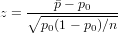
Let us define the test statistic z in terms of the sample proportion and the sample size:

p + Z

\sqrt(p(1-p))/\sqrt(n)

\sqrt(p(1-p))/\sqrt(n)

1-\alpha

1-\alpha

Problem

Suppose 60% of citizens voted in last election. 85 out of 148 people in a telephone survey said that they voted in current election. At 0.5 significance level, can we reject the null hypothesis that the proportion of voters in the population is above 60% this year?

Solution

The null hypothesis is that p ≥ 0.6. We begin with computing the test statistic.

We then compute the critical value at .05 significance level.

> pbar = 85/148          # sample proportion 
> p0 = .6                # hypothesized value 
> n = 148                # sample size 
> z = (pbar−p0)/sqrt(p0∗(1−p0)/n) 
> z                      # test statistic

> alpha = .05 
> z.alpha = qnorm(1−alpha) 
> −z.alpha               # critical value

Answer

The test statistic -0.6376 is not less than the critical value of -1.6449. Hence, at .05 significance level, we do not reject the null hypothesis that the proportion of voters in the population is above 60% this year.

Alternative Solution 1

Instead of using the critical value, we apply the pnorm function to compute the lower tail p-value of the test statistic. As it turns out to be greater than the .05 significance level, we do not reject the null hypothesis thatp ≥ 0.6.

> pval = pnorm(z) 
> pval                   # lower tail p−value

Problem

Suppose that 12% of apples harvested in an orchard last year was rotten. 30 out of 214 apples in a harvest sample this year turns out to be rotten. At .05 significance level, can we reject the null hypothesis that the proportion of rotten apples in harvest stays below 12% this year?

Solution

The null hypothesis is that p ≤ 0.12. We begin with computing the test statistic.

We then compute the critical value at .05 significance level.

> pbar = 30/214          # sample proportion 
> p0 = .12               # hypothesized value 
> n = 214                # sample size 
> z = (pbar−p0)/sqrt(p0∗(1−p0)/n) 
> z                      # test statistic

> alpha = .05 
> z.alpha = qnorm(1−alpha) 
> z.alpha                # critical value

Answer

The test statistic 0.90875 is not greater than the critical value of 1.6449. Hence, at .05 significance level, we do not reject the null hypothesis that the proportion of rotten apples in harvest stays below 12% this year.

Alternative Solution 1

Instead of using the critical value, we apply the pnorm function to compute the upper tail p-value of the test statistic. As it turns out to be greater than the .05 significance level, we do not reject the null hypothesis thatp ≤ 0.12.

pval = pnorm(z, lower.tail=FALSE) 
pval                   # upper tail p−value

Problem

Suppose a coin toss turns up 12 heads out of 20 trials. At .05 significance level, can one reject the null hypothesis that the coin toss is fair?

Solution

The null hypothesis is that p = 0.5. We begin with computing the test statistic.

We then compute the critical values at .05 significance level.

> pbar = 12/20           # sample proportion 
> p0 = .5                # hypothesized value 
> n = 20                 # sample size 
> z = (pbar−p0)/sqrt(p0∗(1−p0)/n) 
> z                      # test statistic

> alpha = .05 
> z.half.alpha = qnorm(1−alpha/2) 
> c(−z.half.alpha, z.half.alpha)

Answer

The test statistic 0.89443 lies between the critical values -1.9600 and 1.9600. Hence, at .05 significance level, we do not reject the null hypothesis that the coin toss is fair.

Alternative Solution 1

Instead of using the critical value, we apply the pnorm function to compute the two-tailed p-value of the test statistic. It doubles the upper tail p-value as the sample proportion is greater than the hypothesized value. Since it turns out to be greater than the .05 significance level, we do not reject the null hypothesis that p = 0.5.

> pval = 2 ∗ pnorm(z, lower.tail=FALSE)  # upper tail 
> pval                   # two−tailed p−value

THANK YOU

Hypothesis Testing

By Rahul Bajaj

Hypothesis Testing

Rahul Bajaj

Data Scientist by Profession - Enjoy number crunching using Open Source Technologies. Feel free to reach out to me at rahulbajaj@hotmail.co.in

Hypothesis

Testing

Problem 1

Problem 1

Solution

Answer

Alternative Solution

Problem 2

Solution

Answer

Alternative Solution

Problem 3

Solution

Answer

Alternative Solution

T Statistic

Student's t-distribution

(or simply t-distribution)

Problem

Solution

Answer

Alternative Solution

Problem

Solution

Answer

Alternative Solution

Problem

Solution

Answer

Alternative Solution

Problem

Solution

Answer

Alternative Solution

Problem

Solution

Answer

Alternative Solution

Problem

Solution

Answer

Alternative Solution

Estimating Proportion

Distribution of Sample Proportion

Distribution of Sample Proportion

Problem

Solution

Answer

Alternative Solution 1

Problem

Solution

Answer

Alternative Solution 1

Problem

Solution

Answer

Alternative Solution 1

Hypothesis Testing

More from Rahul Bajaj