Neural Field Transformations

(for lattice gauge theory)

Sam Foreman

2021-03-11

Introduction

LatticeQCD:
- Non-perturbative approach to solving the QCD theory of the strong interaction between quarks and gluons
Calculations in LatticeQCD proceed in 3 steps:

Gauge field generation: Use Markov Chain Monte Carlo methods for sampling independent gauge field (gluon) configurations.

Propagator calculations: Compute how quarks propagate in these fields ("quark propagators")

Contractions: Method for combining quark propagators into correlation functions and observables.

Markov Chain Monte Carlo (MCMC)

Goal: Draw independent samples from a target distribution, \(p(x)\)

x^{\prime} = x_{0} + \delta,\quad \delta\sim\mathcal{N}(0, \mathbb{1})

Starting from some initial state \(x_{0}\) (randomly chosen), we generate proposal configurations \(x^{\prime}\)

Use Metropolis-Hastings acceptance criteria

x_{i+1} = \begin{cases} x^{\prime},\quad\text{with probability } A(x^{\prime}|x)\\ x,\quad\text{with probability } 1 - A(x^{\prime}|x) \end{cases}

A(x^{\prime}|x) = \min\left\{1, \frac{p(x^{\prime})}{p(x)}\left|\frac{\partial x^{\prime}}{\partial x^{T}}\right|\right\}

Metropolis-Hastings: Accept/Reject

import numpy as np

def metropolis_hastings(p, steps=1000):
    x = 0.                   # initialize config
    samples = np.zeros(steps)
    for i in range(steps):
        x_prime = x + np.random.randn()           # proposed config
        if np.random.rand() < p(x_prime) / p(x):  # compute A(x'|x)
            x = x_prime      # accept proposed config
        samples[i] = x       # accumulate configs 
    
    return samples

N \longrightarrow \infty

x\sim p

Issues with MCMC

Generate proposal configurations
- \(x^{\prime} = x + \delta\), where \(\delta \sim \mathcal{N}(0, \mathbb{1})\)

dropped configurations

Inefficient!

\{x_{0}, x_{1}, x_{2}, \ldots, x_{k}, x_{k+1}, x_{k+2}, x_{k+3}, \ldots, x_{m}, x_{m+1}, x_{m+2}, \ldots, x_{n-2}, x_{n-1}, x_{n}\}

Construct chain:

Account for thermalization ("burn-in"):

\{x_{0}, x_{1}, x_{2}, \ldots, x_{k}, x_{k+1}, x_{k+2}, x_{k+3}, \ldots, x_{m}, x_{m+1}, x_{m+2}, \ldots, x_{n-2}, x_{n-1}, x_{n}\}

Account for correlations between states ("thinning"):

\{x_{0}, x_{1}, x_{2}, \ldots, x_{k}, x_{k+1}, x_{k+2}, x_{k+3}, \ldots, x_{m}, x_{m+1}, x_{m+2}, \ldots, x_{n-2}, x_{n-1}, x_{n}\}

Hamiltonian Monte Carlo (HMC)

Target distribution:

\(p(x)\propto e^{-S(x)}\)

Introduce fictitious momentum:

Joint target distribution, \(p(x, v)\)

\(p(x, v) = p(x)\cdot p(v) = e^{-S(x)}\cdot e^{-\frac{1}{2}v^{T}v} = e^{-\mathcal{H(x,v)}}\)

The joint \((x, v)\) system obeys Hamilton's Equations:

\(v\sim\mathcal{N}(0, 1)\)

\(\dot{x} = \frac{\partial\mathcal{H}}{\partial v}\)

\(\dot{v} = -\frac{\partial\mathcal{H}}{\partial x}\)

\(S(x)\) is the action

(potential energy)

HMC: Leapfrog Integrator

\(\dot{v}=-\frac{\partial\mathcal{H}}{\partial x}\)

\(\dot{x}=\frac{\partial\mathcal{H}}{\partial v}\)

Hamilton's Equations:

v^{1/2} = v - \frac{\varepsilon}{2}\partial_{x}S(x)

x^{\prime} = x + \varepsilon v^{1/2}

v^{\prime} = v^{1/2} - \frac{\varepsilon}{2}\partial_{x}S(x^{\prime})

2. Full-step position update:

1. Half-step momentum update:

3. Half-step momentum update:

\mathcal{H}(x, v) = S(x) + \frac{1}{2}v^{T}v \Longrightarrow

HMC: Issues

Cannot easily traverse low-density zones.

What do we want in a good sampler?

Fast mixing
Fast burn-in

Mix across energy levels
Mix between modes

Energy levels selected randomly \(\longrightarrow\) slow mixing!

(especially for Lattice QCD)

L2HMC: Generalized Leapfrog

Main idea:
- Introduce six auxiliary functions, \((s_{x}, t_{x}, q_{x})\), \((s_{v}, t_{v}, q_{v})\) into the leapfrog updates, which are parameterized by weights \(\theta\) in a neural network.

Notation:
- Introduce a binary direction variable, \(d\sim\mathcal{U}(+,-)\)
  - distributed independently of \(x\), \(v\)
- Denote a complete state by \(\xi = (x, v, d)\), with target distribution \(p(\xi)\):

= p(x, v, d) = p(x)\cdot p(v)\cdot p(d)

p(\xi)

L2HMC: Generalized Leapfrog

Define (\(v\)-independent): \(\zeta_{v_{k}} \equiv (x_{k}, \partial_{x}S(x_{k}), \tau(k))\)

v^{\prime}_{k} \equiv \Gamma^{+}_{k}(v_{k};\zeta_{v_{k}}) = v_{k}\odot \exp\left(\frac{\varepsilon^{k}_{v}}{2}s^{k}_{v}(\zeta_{v_{k}})\right) - \frac{\varepsilon^{k}_{v}}{2}\left[\partial_{x}S(x_{k})\odot\exp\left(\varepsilon^{k}_{v}q^{k}_{v}(\zeta_{v_{k}})\right) + t^{k}_{v}(\zeta_{v_{k}})\right]

\overbrace{\hspace{85px}}

momentum (\(v_{k}\)) scaling

Gradient \(\partial_{x}S(x_{k})\) scaling

\overbrace{\hspace{30px}}

Translation

x^{\prime}_{k} \equiv \Lambda^{+}_{k}(x_{k};\zeta_{x_{k}}) = x_{k}\odot\exp\left(\varepsilon^{k}_{x}s^{k}_{x}(\zeta_{x_{k}})\right) + \varepsilon^{k}_{x}\left[v^{\prime}_{k}\odot\exp\left(\varepsilon^{k}_{x}q^{k}_{x}(\zeta_{x_{k}})\right)+t^{k}_{x}(\zeta_{x_{k}})\right]

\overbrace{\hspace{105px}}

Introduce generalized \(v\)-update, \(v^{\prime}_{k} = \Gamma^{+}_{k}(v_{k};\zeta_{v_{k}})\):

For \(\zeta_{x_{k}} = (x_{k}, v_{k}, \tau(k))\)

And the generalized \(x\)-update, \(x^{\prime}_{k} = \Lambda^{+}_{k}(x_{k};\zeta_{x_{k}})\)

L2HMC: Generalized Leapfrog

Complete (generalized) update:
1. Half-step momentum update:
2. Full-step half-position update:
3. Full-step half-position update:
4. Half-step momentum update:

v^{\prime}_{k} = \Gamma^{\pm}(v_{k};\zeta_{v_{k}})

x^{\prime}_{k} = \hspace{14px}\odot x_{k} + \hspace{14px}\odot \Lambda^{\pm}(x_{k};\zeta_{x_{k}})

\bar{m}^{t}

m^{t}

v^{\prime\prime}_{k} = \Gamma^{\pm}(v^{\prime}_{k};\zeta_{v^{\prime}_{k}})

x^{\prime\prime}_{k} = \hspace{14px}\odot \Lambda^{\pm}_{k}(x^{\prime}_{k};\zeta_{x^{\prime}_{k}}) + \hspace{14px}\odot x^{\prime}_{k}

\bar{m}^{t}

m^{t}

\bar{m}^{t}

m^{t}

=\mathbb{1}

Note:

split via \(m^t\)

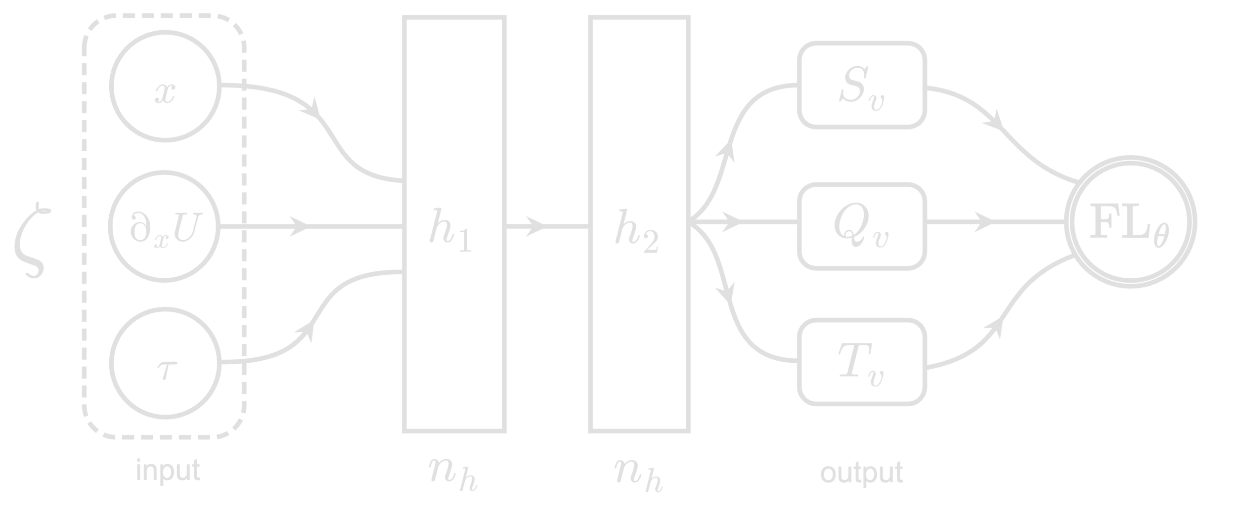
Network Architecture

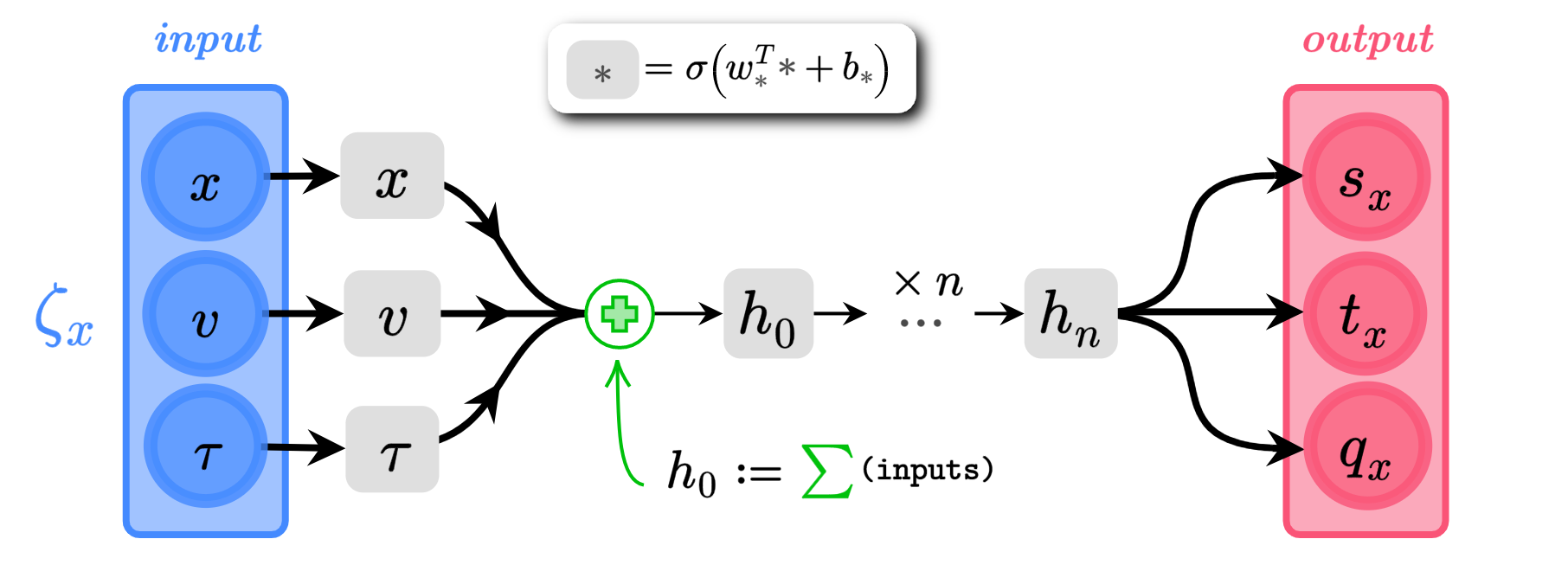
s_{x} = \alpha_{s}\tanh(w^{T}_{s} h_{n} + b_{s})

q_{x} = \alpha_{q}\tanh(w^{T}_{q} h_{n} + b_{q})

t_{x} = w_{t}^{T} h_{n} + b_{t} \in \mathbb{R}^{n}

(\(\alpha_{s}, \alpha_{q}\) are trainable parameters)

\(x\), \(v\) \(\in \mathbb{R}^{n}\)

\(s_{x}\),\(q_{x}\),\(t_{x}\) \(\in \mathbb{R}^{n}\)

Loss function, \(\mathcal{L}(\theta)\)

Goal: Maximize "expected squared jump distance" (ESJD), \(A(\xi^{\prime}|\xi)\cdot \delta(\xi^{\prime}, \xi)\):

\ell_{\theta}\left[\xi^{\prime}, \xi, A(\xi^{\prime}|\xi)\right] = \frac{a^{2}}{A(\xi^{\prime}|\xi)\cdot\delta(\xi^{\prime},\xi)} - \frac{A(\xi^{\prime}|\xi)\cdot\delta(\xi^{\prime},\xi)}{a^{2}}

\delta(\xi^{\prime}, \xi) = \|x^{\prime} - x\|^{2}_{2}

Define the "squared jump distance":

\mathcal{L}_{\theta}\left(\theta\right) \equiv \mathbb{E}_{p(\xi)}\left[\ell_{\theta}\right]

where:

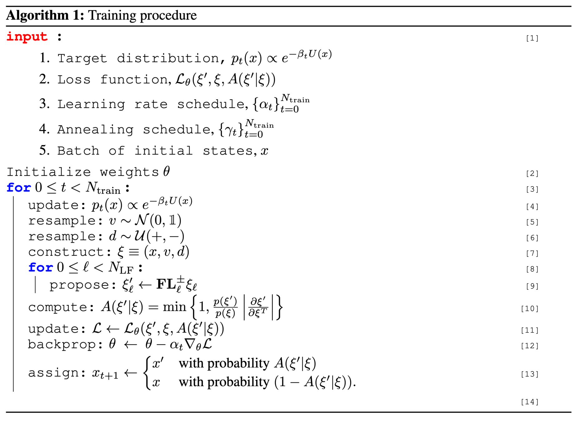
Annealing Schedule

\left\{\gamma_{t}\right\}_{t=0}^{N} = \left\{\gamma_{0}, \gamma_{1}, \ldots, \gamma_{N-1}, \gamma_{N}\right\},

\gamma_{0} < \gamma_{1} < \ldots < \gamma_{N} \equiv 1

\gamma_{t+1} - \gamma_{t} \ll 1

p_{t}(x)\propto e^{-\gamma_{t}S(x)},\quad\text{for}\quad t=0, 1,\ldots, N

Introduce an annealing schedule during the training phase:

For \(\|\gamma_{t}\| < 1\), this helps to rescale (shrink) the energy barriers between isolated modes
- Allows our sampler to explore previously inaccessible regions of the target distribution

Target distribution becomes:

(varied slowly)

\(= \{0.1, 0.2, \ldots, 0.9, 1.0\}\)

(increasing)

L2HMC

HMC

GMM: Autocorrelation

Lattice Gauge Theory

Link variables:

U_{\mu}(x) = e^{i\varphi_{\mu}(x)} \in U(1)

\varphi_{\mu}(x) \in [-\pi,\pi]

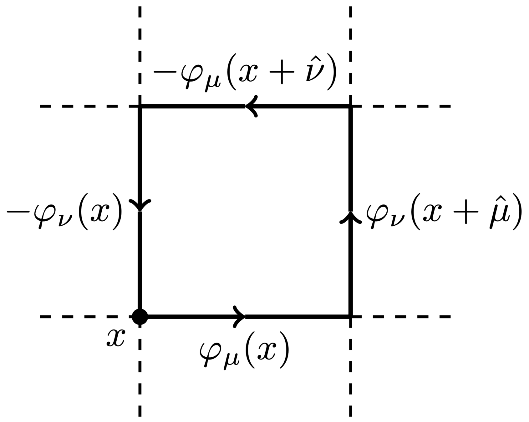
Wilson action:

S(\varphi)=\sum_{P}1-\cos\varphi_{P}

\varphi_{P} = \varphi_{\mu}(x) + \varphi_{\nu}(x+\hat{\mu}) - \varphi_{\mu}(x+\hat{\nu}) - \varphi_{\nu}(x)

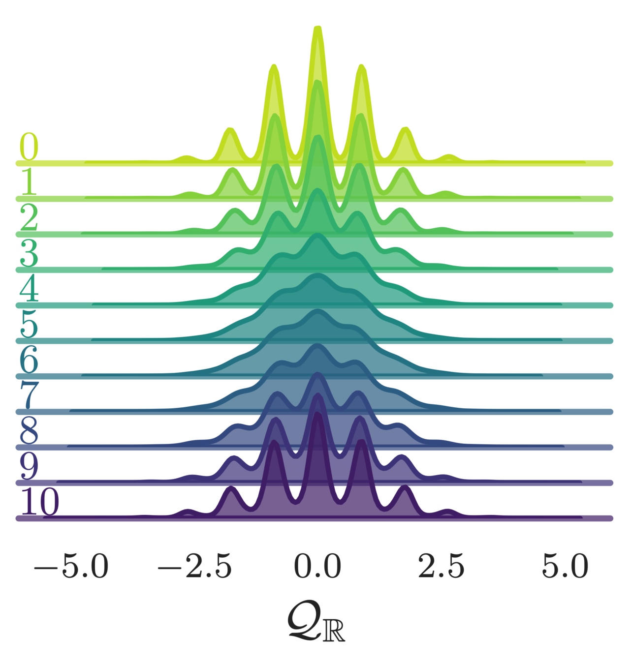
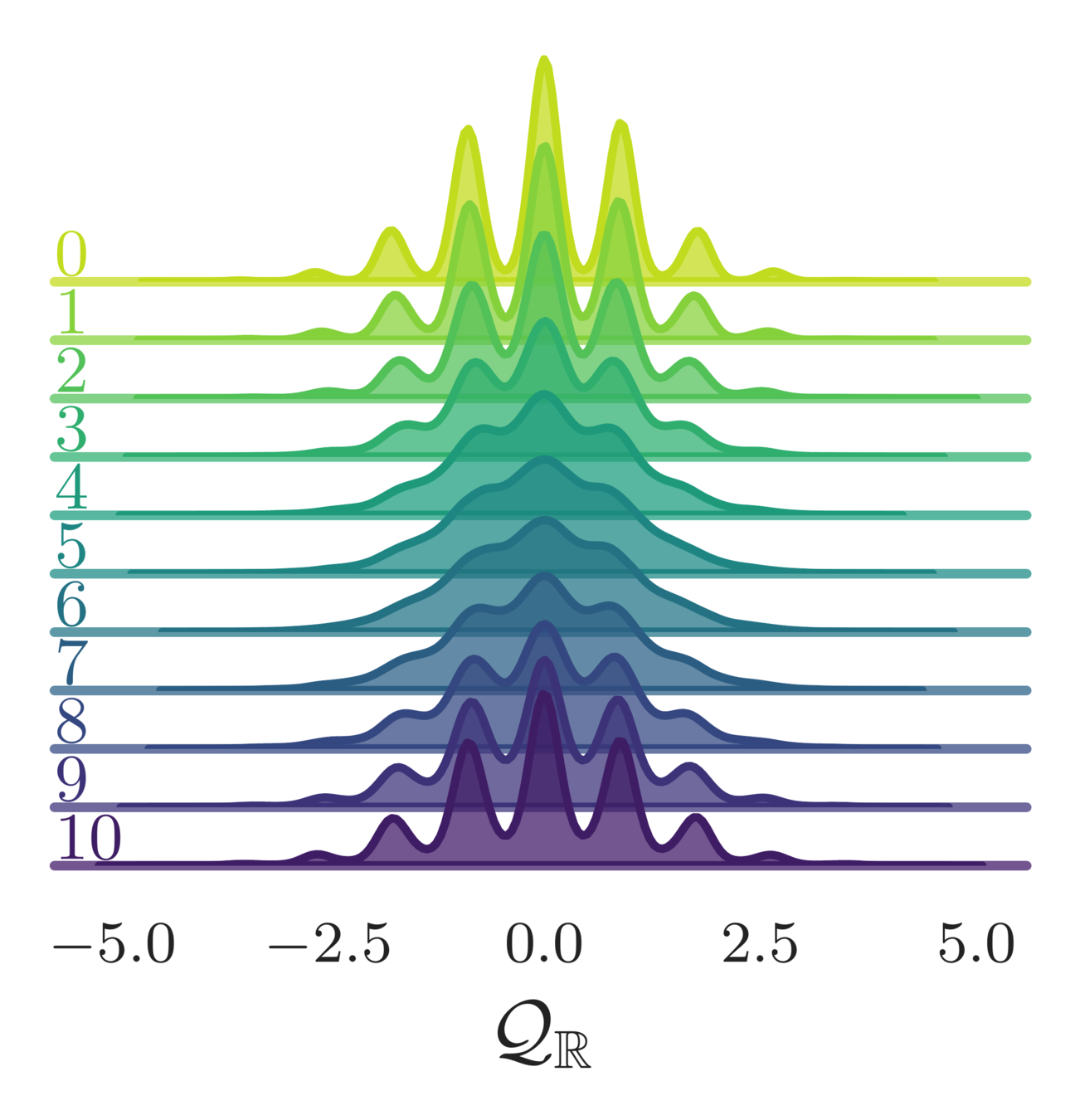
Topological charge:

\mathcal{Q}_{\mathbb{Z}} = \frac{1}{2\pi}\sum_{P}\left\lfloor\varphi_{P}\right\rfloor \in\mathbb{Z},

\left\lfloor\varphi_{P}\right\rfloor = \varphi_{P} - 2\pi\left\lfloor\frac{\varphi_{P}+\pi}{2\pi}\right\rfloor

\mathcal{Q}_{\mathbb{R}} = \frac{1}{2\pi}\sum_{P}\sin\varphi_{P}\in\mathbb{R}

(real-valued)

(integer-valued)

Lattice Gauge Theory

Topological Loss Function:

\ell_{\theta}(\xi^{\prime}, \xi, A(\xi^{\prime}|\xi)) = -\frac{1}{a^{2}}A(\xi^{\prime}|\xi)\cdot \delta_{\mathcal{Q}_{\mathbb{R}}}(\xi^{\prime}, \xi)

\delta_{\mathcal{Q}_{\mathbb{R}}}(\xi^{\prime}, \xi) \equiv \left(\mathcal{Q}_{\mathbb{R}}^{\prime} - \mathcal{Q}_{\mathbb{R}}\right)^{2}

= \left(\mathcal{Q}_{\mathbb{R}}(\xi^{\prime}) - \mathcal{Q}_{\mathbb{R}}(\xi)\right)^{2}

\(A(\xi^{\prime}|\xi) = \) "acceptance probability"

where:

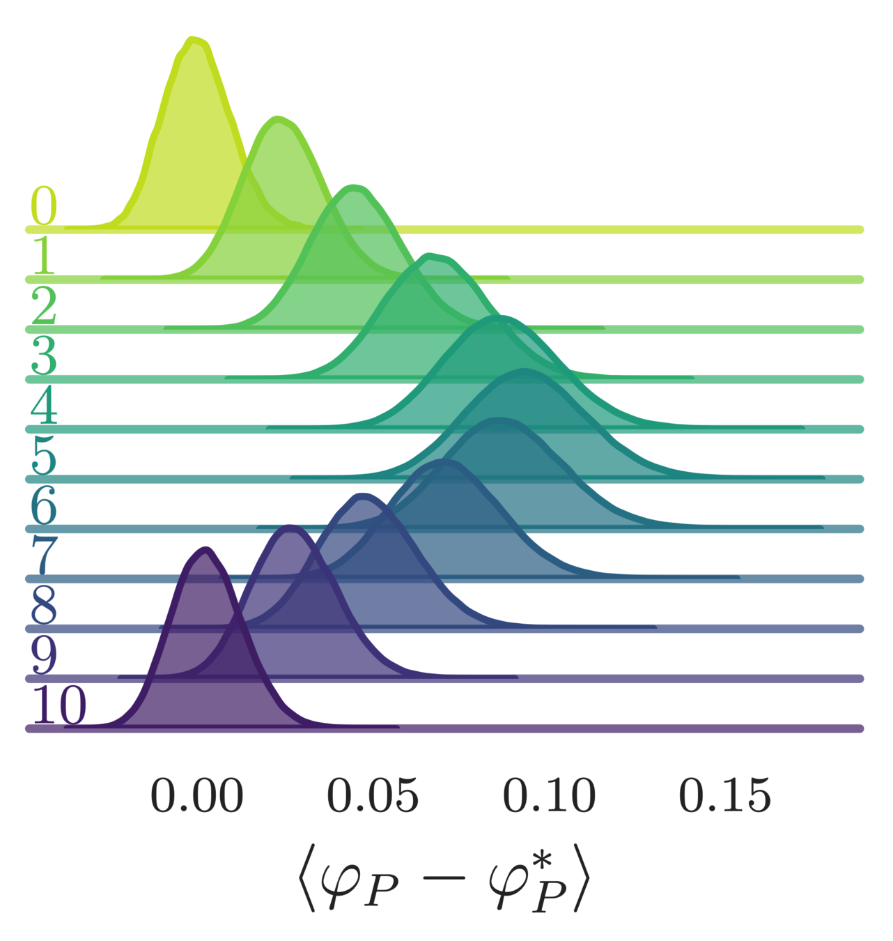
Lattice Gauge Theory

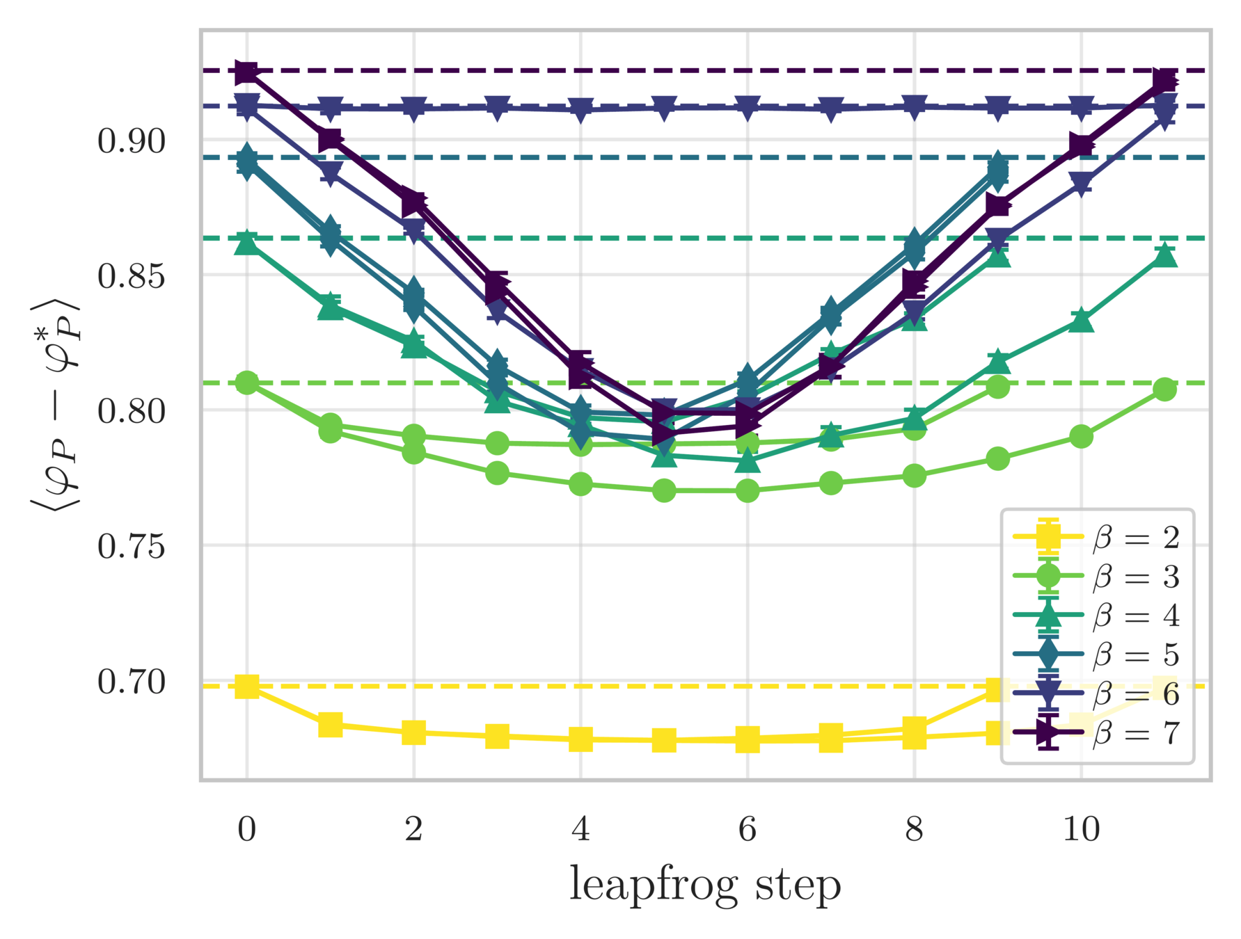
Error in the average plaquette, \(\langle\varphi_{P}-\varphi^{*}\rangle\)
- where \(\varphi^{*} = I_{1}(\beta)/I_{0}(\beta)\) is the exact (\(\infty\)-volume) result

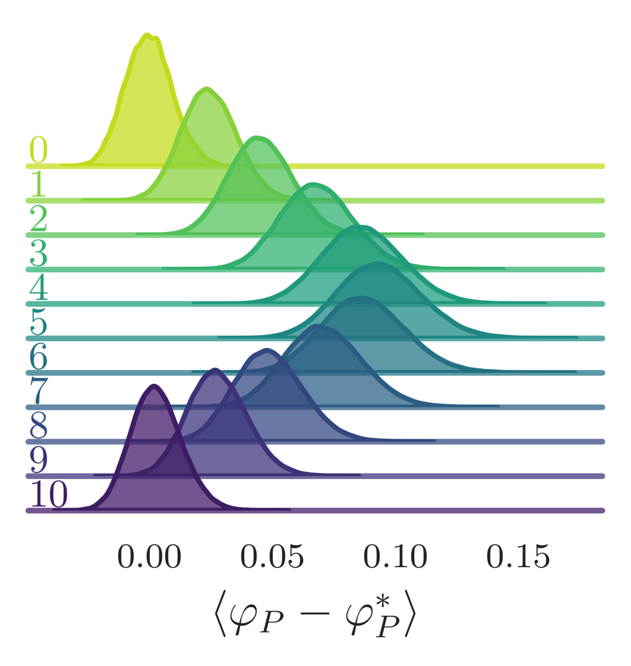
leapfrog step

(MD trajectory)

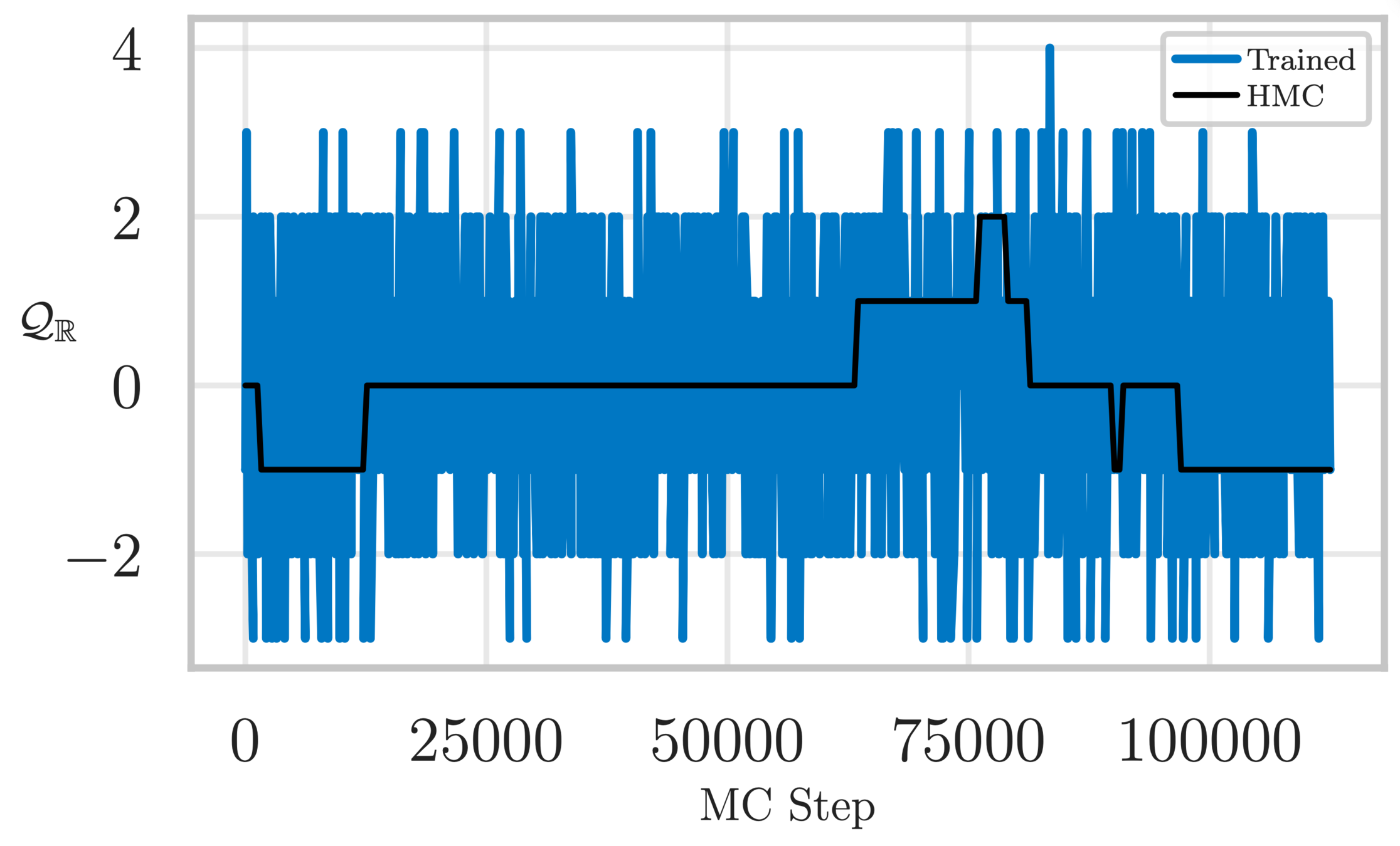
Topological charge history

~ cost / step

continuum limit

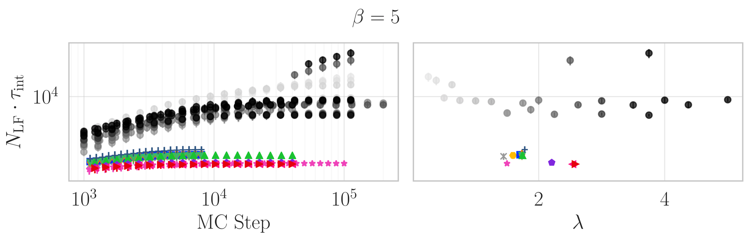
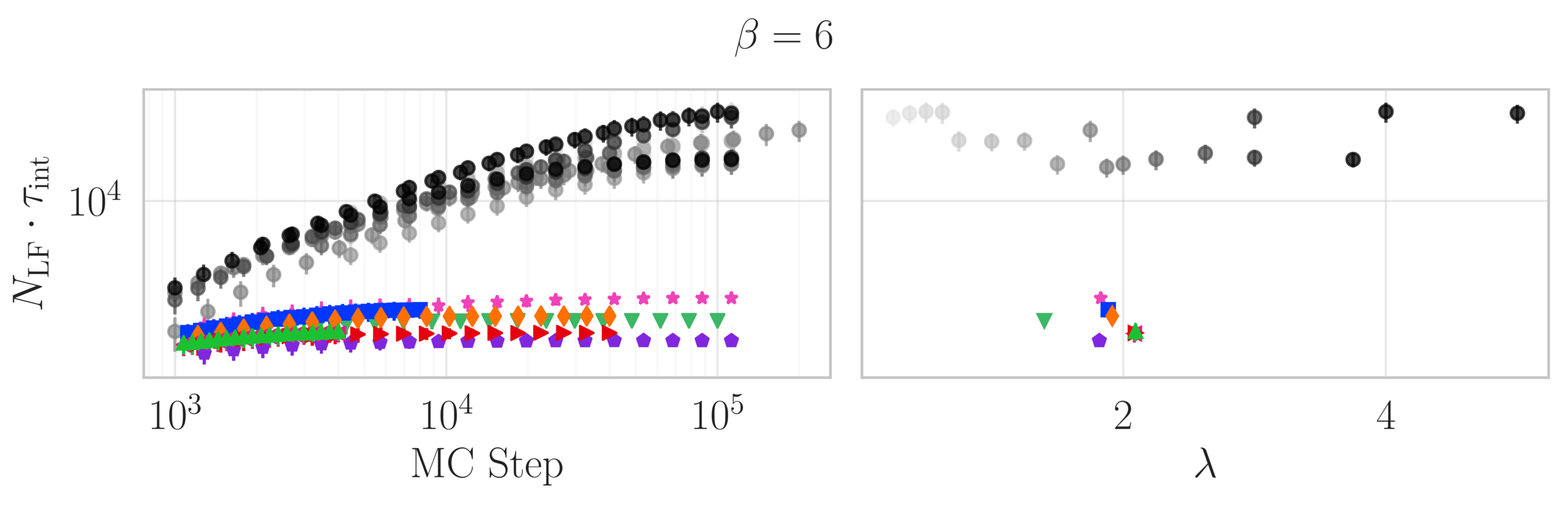
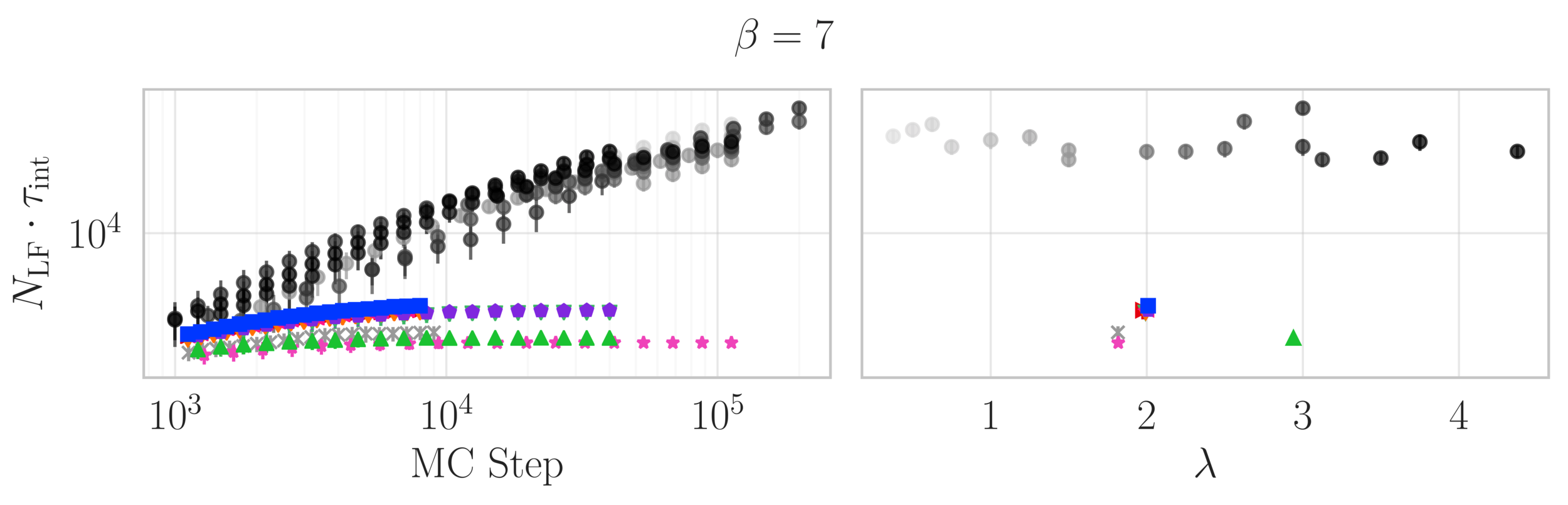
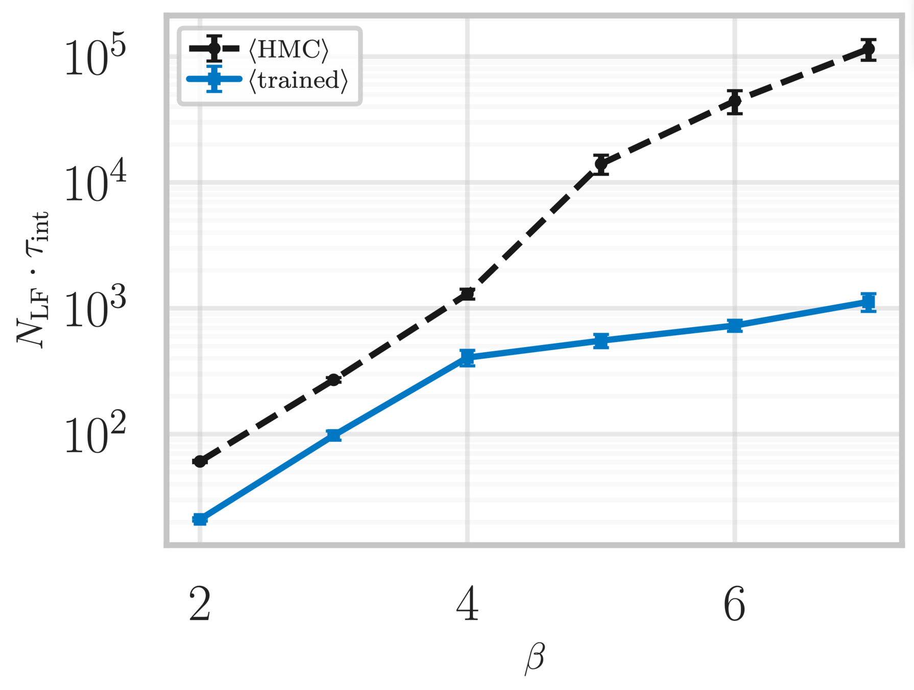
Estimate of the Integrated autocorrelation time of \(\mathcal{Q}_{\mathbb{R}}\)

4096

8192

1024

2048

512

Scaling test: Training

\(4096 \sim 1.73\times\)

\(8192 \sim 2.19\times\)

\(1024 \sim 1.04\times\)

\(2048 \sim 1.29\times\)

\(512\sim 1\times\)

Scaling test: Training

\(8192\sim \times\)

4096

1024

2048

512

Scaling test: Inference

L2HMC: Generalized Leapfrog

Define (\(v\)-independent): \(\zeta_{v_{k}} \equiv (x_{k}, \partial_{x}S(x_{k}), \tau(k))\)

\overbrace{\hspace{85px}}

Momentum scaling

Gradient scaling

\overbrace{\hspace{30px}}

Translation

\overbrace{\hspace{105px}}

Introduce generalized \(v\)-update, \(\Gamma^{+}_{k}(v_{k};\zeta_{v_{k}})\):

Define (\(x\)-independent): \(\zeta_{x_{k}} = (x_{k}, v_{k}, \tau(k))\)

Introduce generalized \(x\)-update, \(\Lambda^{+}_{k}(x_{k};\zeta_{x_{k}})\)

momentum

position

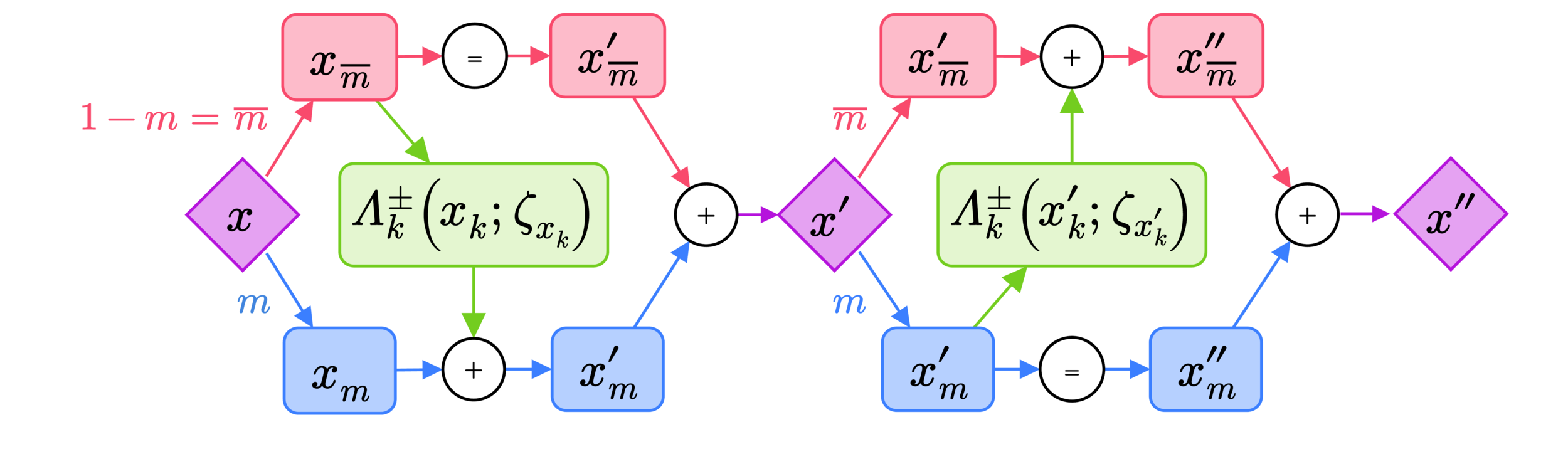
L2HMC: Modified Leapfrog

Split the position, \(x\), update into two sub-updates:
- Introduce a binary mask \(m^{t} \in\{0, 1\}^{n}\) and its complement \(\bar{m}^{t}\).
- \(m^{t}\) is drawn uniformly from the set of binary vectors satisfying \(\sum_{i=1}^{n}m_{i}^{t} = \lfloor{\frac{n}{2}\rfloor}\) (i.e. half of the entries of \(m^{t}\) are 0 and half are 1.)

Introduce a binary direction variable \(d \in \{-1, 1\}\), drawn from a uniform distribution.
- Denote the complete augmented state as \(\xi \equiv (x, v, d)\).

(forward direction, \(d = +1\))

v_{k}^{\prime} = v\odot\exp\left(\frac{\varepsilon^{k}_{v}}{2}s^{k}_{v}(\zeta_{v_{k}})\right) - \frac{\varepsilon^{k}_{v}}{2}\left[\partial_{x}U(x)\odot\exp(\varepsilon^{k}_{v} q^{k}_{v}(\zeta_{v_{k}})) + t^{k}_{v}(\zeta_{v_{k}})\right]

x_{k}^{\prime} = x^{k}_{\bar{m}^{t}} + m^{t}\odot\left[x^{k}\odot \exp(\varepsilon^{k}_{x} s^{k}_{x}(\zeta_{x_{k}})) + \varepsilon^{k}_{x}\left(v^{\prime} \odot\exp(\varepsilon^{k}_{x} q^{k}_{x}(\zeta_{x_{k}})) + t^{k}_{x}(\zeta_{x_{k}})\right)\right]

x_{k}^{\prime\prime} = x_{\bar{m}^{t}}^{\prime} + \bar{m}^{t}\odot\left[x^{\prime}\odot \exp(\varepsilon S_{x}(\zeta_{3})) + \varepsilon\left(v^{\prime} \odot\exp(\varepsilon Q_{x}(\zeta_{3})) + T_{x}(\zeta_{3})\right)\right]

v_{k}^{\prime\prime} = v^{\prime}\odot\exp\left(\frac{\varepsilon}{2}S_{v}(\zeta_{4})\right) - \frac{\varepsilon}{2}\left[\partial_{x}U(x^{\prime\prime})\odot\exp(\varepsilon Q_{v}(\zeta_{4})) + T_{v}(\zeta_{4})\right]

\zeta_{1} = (x, \partial_{x}U(x), t)

\zeta_{2} = (x_{\bar{m}^{t}}, v, t)

\zeta_{3} = (x^{\prime}_{m^{t}}, v, t)

\zeta_{4} = (x^{\prime\prime}, \partial_{x}U(x^{\prime\prime}), t)

\overbrace{\hspace{35px}}

Momentum scaling

\overbrace{\hspace{43px}}

Gradient scaling

\overbrace{\hspace{5px}}

Translation

inputs

L2HMC: Modified Leapfrog

Writing the action of the new leapfrog integrator as an operator \(\mathbf{L}_{\theta}\), parameterized by \(\theta\).

Applying this operator \(M\) times successively to \(\xi\):

\mathbf{L}_{\theta} = \mathbf{L}_{\theta}(x, v, d) = \left(x^{{\prime\prime}^{\times M}}, v^{{\prime\prime}^{\times M}}, d\right)

The "flip" operator \(\mathbf{F}\) reverses \(d\): \(\mathbf{F}\xi = (x, v, -d)\).

Write the complete dynamics step as:

\mathbf{FL}_{\theta} \xi = \xi^{\prime}

(trajectory length)

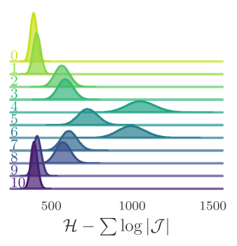
L2HMC: Accept/Reject

Fortunately, the Jacobian can be computed efficiently, and only depends on \(S_{x}, S_{v}\) and all the state variables, \(\zeta_{i}\).

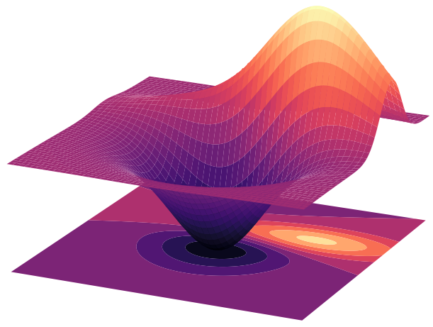
This has the effect of deforming the energy landscape:

\mathcal{J}

Accept the proposed configuration, \(\xi^{\prime}\) with probability:

\(A(\xi^{\prime}|\xi) = \min{\left(1, \frac{p(\mathbf{FL}_{\theta}\xi)}{p(\xi)}\left|\frac{\partial\left[\mathbf{FL}\xi\right]}{\partial\xi^{T}}\right|\right)}\)

\(|\mathcal{J}| \neq 1\)

Unlike HMC,

L2HMC: Loss function

\ell_{\lambda}\left(\xi, \xi^{\prime}, A(\xi^{\prime}|\xi)\right) = \frac{\lambda^{2}}{\delta(\xi, \xi^{\prime})A(\xi^{\prime}|\xi)} - \frac{\delta(\xi, \xi^{\prime})A(\xi^{\prime}|\xi)}{\lambda^{2}}

\underbrace{\hspace{38px}}

Encourages typical moves to be large

\overbrace{\hspace{38px}}

Penalizes sampler if unable to move effectively

scale parameter

"distance" between \(\xi, \xi^{\prime}\): \(\delta(\xi, \xi^{\prime}) = \|x - x^{\prime}\|^{2}_{2}\)

Idea: MINIMIZE the autocorrelation time (time needed for samples to be independent).
- Done by MAXIMIZING the "distance" traveled by the integrator.

Note:

\(\delta \times A = \) "expected" distance

MCMC in Lattice QCD

Generating independent gauge configurations is a MAJOR bottleneck for LatticeQCD.

As the lattice spacing, \(a \rightarrow 0\), the MCMC updates tend to get stuck in sectors of fixed gauge topology.
- This causes the number of steps needed to adequately sample different topological sectors to increase exponentially.

Critical slowing down!

L2HMC: \(U(1)\) Lattice Gauge Theory

U_{\mu}(i) = e^{i \phi_{\mu}(i)} \in U(1)

-\pi < \phi_{\mu}(i) \leq \pi

\beta S = \beta \sum_{P}\left(1 - \cos(\phi_{P})\right)

Wilson action:

\phi_{P} \equiv \phi_{\mu\nu}(i)\\

= \phi_{\mu}(i) + \phi_{\nu}(i + \hat{\mu})- \phi_{\mu}(i+\hat{\nu}) - \phi_{\nu}(i)

where:

L2HMC: \(U(1)\) Lattice Gauge Theory

U_{\mu}(i) = e^{i \phi_{\mu}(i)} \in U(1)

-\pi < \phi_{\mu}(i) \leq \pi

\beta S = \beta \sum_{P}\left(1 - \cos(\phi_{P})\right)

Wilson action:

\phi_{P} \equiv \phi_{\mu\nu}(i)\\

= \phi_{\mu}(i) + \phi_{\nu}(i + \hat{\mu})- \phi_{\mu}(i+\hat{\nu}) - \phi_{\nu}(i)

where:

L2HMC

HMC

L2HMC

HMC

Thanks for listening!

Interested?

github.com/saforem2/l2hmc-qcd

Machine Learning in Lattice QCD

Sam Foreman

02/10/2020

Network Architecture

Build model,

initialize network

Run dynamics, Accept/Reject

Calculate

Backpropagate

Finished

training?

Save trained

model

Run inference

on saved model

\ell_{\lambda}(\theta)

Train step

Hamiltonian Monte Carlo (HMC)

Integrating Hamilton's equations allows us to move far in state space while staying (roughly) on iso-probability contours of \(p(x, v)\)

Integrate \(H(x, v)\):

\(t \longrightarrow t + \varepsilon\)

Project onto target parameter space \(p(x, v) \longrightarrow p(x)\)

\(v \sim p(v)\)

Markov Chain Monte Carlo (MCMC)

Goal: Generate an ensemble of independent samples drawn from the desired target distribution \(p(x)\).

This is done using the Metropolis-Hastings accept/reject algorithm:

Given:
- Initial distribution, \(\pi_{0}\)
- Proposal distribution, \(q(x^{\prime}|x)\)
Update:
1. Sample \(x^{\prime} \sim q(\cdot | x)\)
2. Accept \(x^{\prime}\) with probability \(A(x^{\prime}|x)\)

A(x^{\prime}|x) = \min\left[1, \frac{p(x^{\prime})q(x|x^{\prime})}{p(x)q(x^{\prime}|x)}\right] = \min\left[1, \frac{p(x^{\prime})}{p(x)}\right]

if \(q(x^{\prime}|x) = q(x|x^{\prime})\)

\longrightarrow

HMC: Leapfrog Integrator

Integrate Hamilton's equations numerically using the leapfrog integrator.

The leapfrog integrator proceeds in three steps:

\dot x_{i} = \frac{\partial\mathcal{H}}{\partial v_{i}} = v_i

\dot v_{i} =-\frac{\partial\mathcal{H}}{\partial x_{i}} = -\frac{\partial U}{\partial x_{i}}

Update momenta (half step):

Update position (full step):

Update momenta (half step):

(1.)

(2.)

(3.)

(t \longrightarrow t + \frac{\varepsilon}{2})

(t \longrightarrow t + \varepsilon)

(t + \frac{\varepsilon}{2} \longrightarrow t + \varepsilon)

v(t + \frac{\varepsilon}{2}) = v(t) - \frac{\varepsilon}{2}\partial_{x} U(x(t))

x(t + \varepsilon) = x(t) + \varepsilon v(t+\frac{\varepsilon}{2})

v(t+\varepsilon) = v(t+\frac{\varepsilon}{2}) - \frac{\varepsilon}{2}\partial_{x}U(x(t+\varepsilon))

Issues with MCMC

Need to wait for the chain to "burn in" (become thermalized)

Nearby configurations on the chain are correlated with each other.
- Multiple steps needed to produce independent samples ("mixing time")
  - Measurable via integrated autocorrelation time, \(\tau^{\mathrm{int}}_{\mathcal{O}}\)

Smaller \(\tau^{\mathrm{int}}_{\mathcal{O}}\longrightarrow\) less computational cost!

correlated!

burn-in

\underbrace{\hspace96px}

\sim p(x)

\overbrace{\hspace 72px}

L2HMC: Learning to HMC

L2HMC generalizes HMC by introducing 6 new functions, \(S_{\ell}, T_{\ell}, Q_{\ell}\), for \(\ell = x, v\) into the leapfrog integrator.

Given an analytically described distribution, L2HMC provides a statistically exact sampler, with highly desirable properties:

Fast burn-in.
Fast mixing.

Ideal for lattice QCD due to critical slowing down!

Idea: MINIMIZE the autocorrelation time (time needed for samples to be independent).
- Can be done by MAXIMIZING the "distance" traveled by the integrator.

HMC: Leapfrog Integrator

Write the action of the leapfrog integrator in terms of an operator \(L\), acting on the state \(\xi \equiv (x, v)\):

\mathbf{L}\xi \equiv \mathbf{L}(x, v)\equiv (x^{\prime}, v^{\prime})

\mathbf{F}\xi \equiv \mathbf{F}(x, v) \equiv (x, -v)

The acceptance probability is then given by:

Introduce a "momentum-flip" operator, \(\mathbf{F}\):

A\left(\xi^{\prime}|\xi\right) = \min\left(1, \frac{p(\xi^{\prime})}{p(\xi)}\left|\frac{\partial\left[\xi^{\prime}\right]}{\partial\xi^{T}}\right|\right)

Determinant of the Jacobian, \(\|\mathcal{J}\|\)

(for HMC)

L2HMC: Generalized Leapfrog

Define (\(v\)-independent): \(\zeta_{v_{k}} \equiv (x_{k}, \partial_{x}S(x_{k}), \tau(k))\)

\overbrace{\hspace{85px}}

Momentum scaling

Gradient scaling

\overbrace{\hspace{30px}}

Translation

\overbrace{\hspace{105px}}

Introduce generalized \(v\)-update, \(\Gamma^{+}_{k}(v_{k};\zeta_{v_{k}})\):

For \(\zeta_{x_{k}} = (x_{k}, v_{k}, \tau(k))\)

And the generalized \(x\)-update, \(\Lambda^{+}_{k}(x_{k};\zeta_{x_{k}})\)

momentum

position

l2hmc-qcd (w/ extra slides)

By Sam Foreman

l2hmc-qcd (w/ extra slides)

Machine Learning in Lattice QCD

Sam Foreman

saforem2

Neural Field Transformations

(for lattice gauge theory)

Introduction

LatticeQCD:

Calculations in LatticeQCD proceed in 3 steps:

Markov Chain Monte Carlo (MCMC)

Issues with MCMC

Hamiltonian Monte Carlo (HMC)

HMC: Leapfrog Integrator

\(\dot{v}=-\frac{\partial\mathcal{H}}{\partial x}\)

\(\dot{x}=\frac{\partial\mathcal{H}}{\partial v}\)

HMC: Issues

L2HMC: Generalized Leapfrog

L2HMC: Generalized Leapfrog

L2HMC: Generalized Leapfrog

Network Architecture

Loss function, \(\mathcal{L}(\theta)\)

Annealing Schedule

L2HMC

HMC

GMM: Autocorrelation

Lattice Gauge Theory

Lattice Gauge Theory

Lattice Gauge Theory

Scaling test: Training

Scaling test: Training

Scaling test: Training

Scaling test: Inference

L2HMC: Generalized Leapfrog

L2HMC: Modified Leapfrog

L2HMC: Modified Leapfrog

L2HMC: Accept/Reject

L2HMC: Loss function

MCMC in Lattice QCD

Critical slowing down!

L2HMC: \(U(1)\) Lattice Gauge Theory

Wilson action:

L2HMC: \(U(1)\) Lattice Gauge Theory

Wilson action:

L2HMC

HMC

L2HMC

HMC

Thanks for listening!

Machine Learning in Lattice QCD

Sam Foreman

Network Architecture

Hamiltonian Monte Carlo (HMC)

HMC: Leapfrog Integrator

Update momenta (half step):

Update position (full step):

Update momenta (half step):

Issues with MCMC

Smaller \(\tau^{\mathrm{int}}_{\mathcal{O}}\longrightarrow\) less computational cost!

L2HMC: Learning to HMC

HMC: Leapfrog Integrator

L2HMC: Generalized Leapfrog

l2hmc-qcd (w/ extra slides)

More from Sam Foreman