Neural Field Transformations
(for lattice gauge theory)
Sam Foreman
2021-03-11

Introduction
-
LatticeQCD:
- Non-perturbative approach to solving the QCD theory of the strong interaction between quarks and gluons
-
Calculations in LatticeQCD proceed in 3 steps:
- Gauge field generation: Use Markov Chain Monte Carlo (MCMC) methods for sampling independent gauge field (gluon) configurations.
- Propagator calculations: Compute how quarks propagate in these fields ("quark propagators")
- Contractions: Method for combining quark propagators into correlation functions and observables.
Motivation: Lattice QCD
- Generating independent gauge configurations is a major bottleneck in the HEP/LatticeQCD workflow
- As the lattice spacing \(a\rightarrow 0\), configurations get stuck
stuck
\(a\)
continuum limit
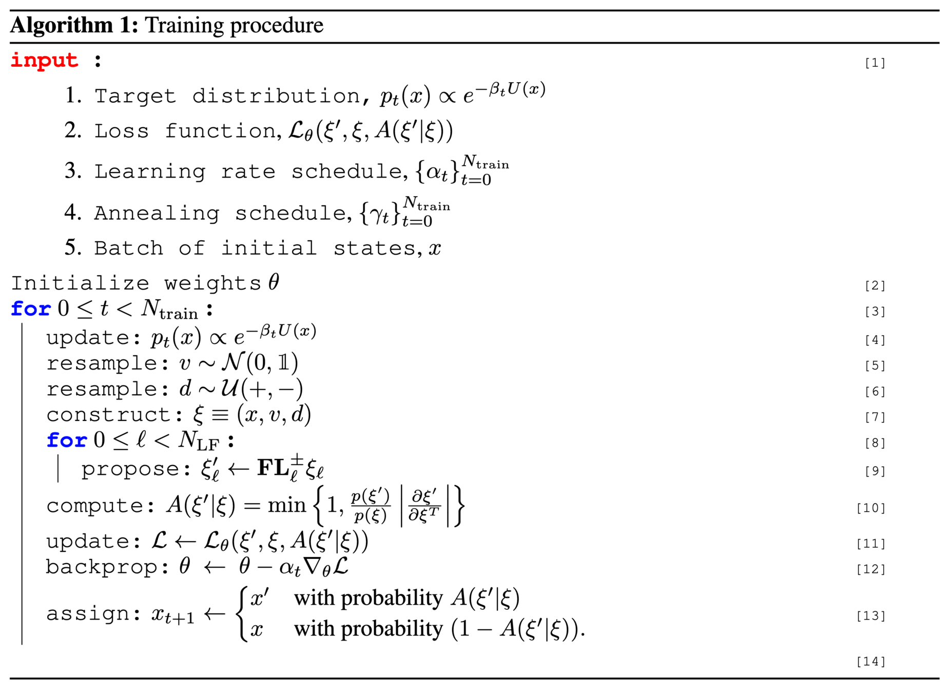
Markov Chain Monte Carlo (MCMC)
- Goal: Draw independent samples from a target distribution, \(p(x)\)
x^{\prime} = x_{0} + \delta,\quad \delta\sim\mathcal{N}(0, \mathbb{1})
- Starting from some initial state \(x_{0}\) (randomly chosen), we generate proposal configurations \(x^{\prime}\)
- Use Metropolis-Hastings acceptance criteria
x_{i+1} =
\begin{cases}
x^{\prime},\quad\text{with probability } A(x^{\prime}|x)\\
x,\quad\text{with probability } 1 - A(x^{\prime}|x)
\end{cases}
A(x^{\prime}|x) = \min\left\{1, \frac{p(x^{\prime})}{p(x)}\left|\frac{\partial x^{\prime}}{\partial x^{T}}\right|\right\}
Metropolis-Hastings: Accept/Reject
import numpy as np

def metropolis_hastings(p, steps=1000):
    x = 0.                   # initialize config
    samples = np.zeros(steps)
    for i in range(steps):
        x_prime = x + np.random.randn()           # proposed config
        if np.random.rand() < p(x_prime) / p(x):  # compute A(x'|x)
            x = x_prime      # accept proposed config
        samples[i] = x       # accumulate configs

    return samples


N \longrightarrow \infty
As
x\sim p
,
Issues with MCMC
- Generate proposal configurations
dropped configurations
Inefficient!
\{x_{0}, x_{1}, x_{2}, \ldots, x_{k}, x_{k+1}, x_{k+2}, x_{k+3}, \ldots, x_{m}, x_{m+1}, x_{m+2}, \ldots, x_{n-2}, x_{n-1}, x_{n}\}
- Construct chain:
- Account for thermalization ("burn-in"):
\{x_{0}, x_{1}, x_{2}, \ldots, x_{k}, x_{k+1}, x_{k+2}, x_{k+3}, \ldots, x_{m}, x_{m+1}, x_{m+2}, \ldots, x_{n-2}, x_{n-1}, x_{n}\}
- Account for correlations between states ("thinning"):
\{x_{0}, x_{1}, x_{2}, \ldots, x_{k}, x_{k+1}, x_{k+2}, x_{k+3}, \ldots, x_{m}, x_{m+1}, x_{m+2}, \ldots, x_{n-2}, x_{n-1}, x_{n}\}
x^{\prime} = x + \delta, \quad\text{where}\quad \delta \sim \mathcal{N}(0, \mathbb{1})
Hamiltonian Monte Carlo (HMC)
-
Target distribution:
\(p(x)\propto e^{-S(x)}\)
-
Introduce fictitious momentum:
-
Joint target distribution, \(p(x, v)\)
\(p(x, v) = p(x)\cdot p(v) = e^{-S(x)}\cdot e^{-\frac{1}{2}v^{T}v} = e^{-\mathcal{H(x,v)}}\)
-
The joint \((x, v)\) system obeys Hamilton's Equations:
\(v\sim\mathcal{N}(0, 1)\)
\(\dot{x} = \frac{\partial\mathcal{H}}{\partial v}\)
\(\dot{v} = -\frac{\partial\mathcal{H}}{\partial x}\)
\(S(x)\) is the action
(potential energy)
HMC: Leapfrog Integrator
\(\dot{v}=-\frac{\partial\mathcal{H}}{\partial x}\)
\(\dot{x}=\frac{\partial\mathcal{H}}{\partial v}\)
Hamilton's Equations:
v^{1/2} = v - \frac{\varepsilon}{2}\partial_{x}S(x)
x^{\prime} = x + \varepsilon v^{1/2}
v^{\prime} = v^{1/2} - \frac{\varepsilon}{2}\partial_{x}S(x^{\prime})
2. Full-step position update:
1. Half-step momentum update:
3. Half-step momentum update:
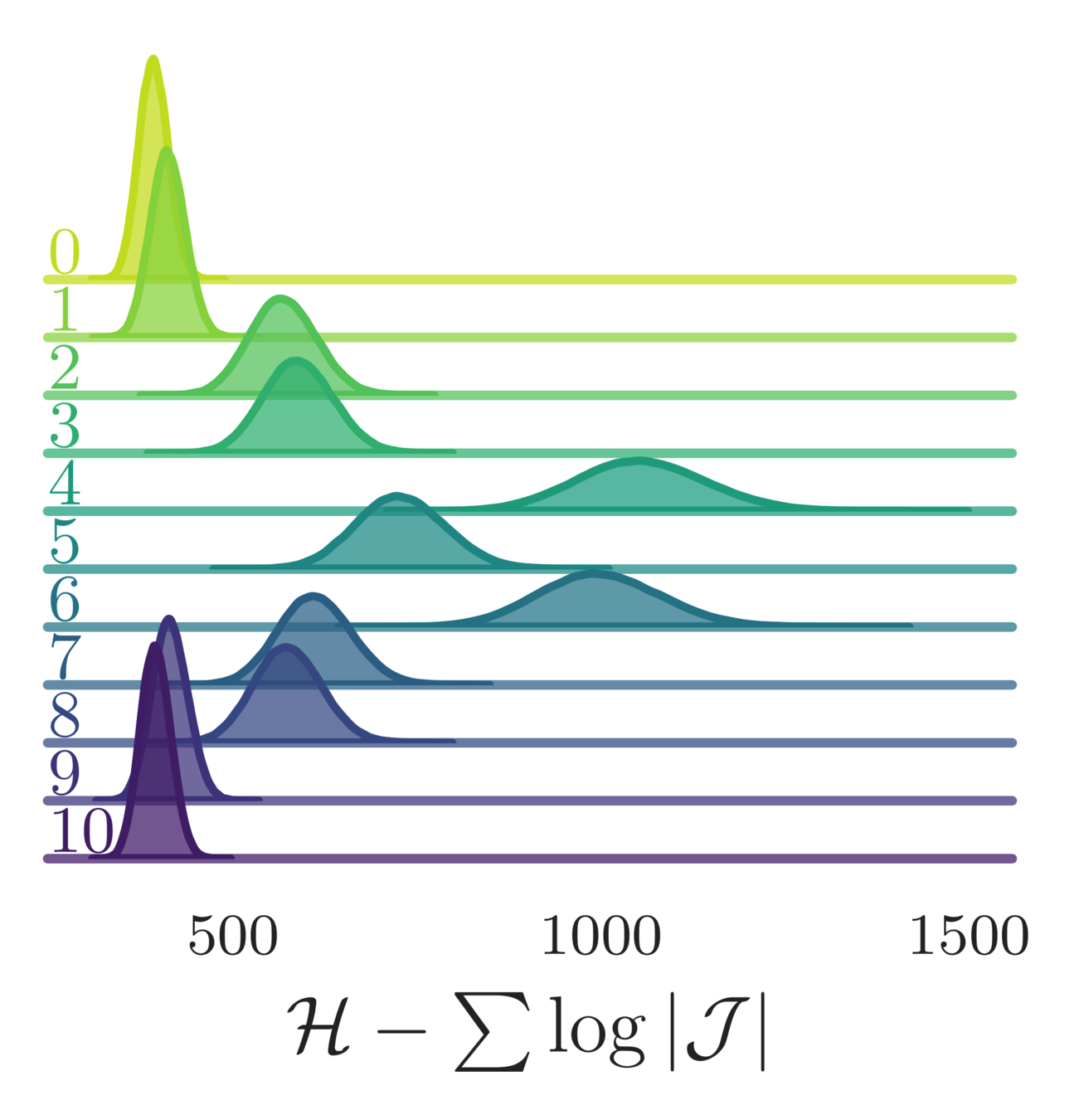
\mathcal{H}(x, v) = S(x) + \frac{1}{2}v^{T}v \Longrightarrow
HMC: Issues
-
Cannot easily traverse low-density zones.
-
\(A(\xi^{\prime}|\xi)\approx 0\)
-
-
What do we want in a good sampler?
- Fast mixing
- Fast burn-in
- Mix across energy levels
- Mix between modes
-
Energy levels selected randomly
-
\(v\sim \mathcal{N}(0, 1)\) \(\longrightarrow\) slow mixing!
-
(especially for Lattice QCD)
L2HMC: Generalized Leapfrog
-
Main idea:
- Introduce six auxiliary functions, \((s_{x}, t_{x}, q_{x})\), \((s_{v}, t_{v}, q_{v})\) into the leapfrog updates, which are parameterized by weights \(\theta\) in a neural network.
-
Notation:
-
Introduce a binary direction variable, \(d\sim\mathcal{U}(+,-)\)
- distributed independently of \(x\), \(v\)
- Denote a complete state by \(\xi = (x, v, d)\), with target distribution \(p(\xi)\):
-
Introduce a binary direction variable, \(d\sim\mathcal{U}(+,-)\)
= p(x, v, d) = p(x)\cdot p(v)\cdot p(d)
p(\xi)
L2HMC: Generalized Leapfrog
v^{\prime}_{k} \equiv \Gamma^{+}_{k}(v_{k};\zeta_{v_{k}}) = v_{k}\odot \exp\left(\frac{\varepsilon^{k}_{v}}{2}s^{k}_{v}(\zeta_{v_{k}})\right) - \frac{\varepsilon^{k}_{v}}{2}\left[\partial_{x}S(x_{k})\odot\exp\left(\varepsilon^{k}_{v}q^{k}_{v}(\zeta_{v_{k}})\right) + t^{k}_{v}(\zeta_{v_{k}})\right]
\overbrace{\hspace{85px}}
Momentum scaling
Gradient scaling
\overbrace{\hspace{30px}}
Translation
x^{\prime}_{k} \equiv \Lambda^{+}_{k}(x_{k};\zeta_{x_{k}}) = x_{k}\odot\exp\left(\varepsilon^{k}_{x}s^{k}_{x}(\zeta_{x_{k}})\right) + \varepsilon^{k}_{x}\left[v^{\prime}_{k}\odot\exp\left(\varepsilon^{k}_{x}q^{k}_{x}(\zeta_{x_{k}})\right)+t^{k}_{x}(\zeta_{x_{k}})\right]
\overbrace{\hspace{105px}}
momentum
position
- Introduce generalized \(v\)-update, \(v^{\prime}_{k} = \Gamma^{+}_{k}(v_{k};\zeta_{v_{k}})\):
with \(\zeta_{x_{k}} = (x_{k}, v_{k}, \tau(k))\)
- And the generalized \(x\)-update, \(x^{\prime}_{k} = \Lambda^{+}_{k}(x_{k};\zeta_{x_{k}})\)
with (\(v\)-independent) \(\zeta_{v_{k}} \equiv (x_{k}, \partial_{x}S(x_{k}), \tau(k))\)
L2HMC: Generalized Leapfrog
- Complete (generalized) update:
- Half-step momentum update:
- Full-step half-position update:
- Full-step half-position update:
- Half-step momentum update:
v^{\prime}_{k} = \Gamma^{\pm}_{k}(v_{k};\zeta_{v_{k}})
x^{\prime}_{k} = \hspace{14px}\odot\, x_{k} + \hspace{14px}\odot\, \Lambda^{\pm}_{k}(x_{k};\zeta_{x_{k}})
\bar{m}^{t}
m^{t}
v^{\prime\prime}_{k} = \Gamma^{\pm}_{k}(v^{\prime}_{k};\zeta_{v^{\prime}_{k}})
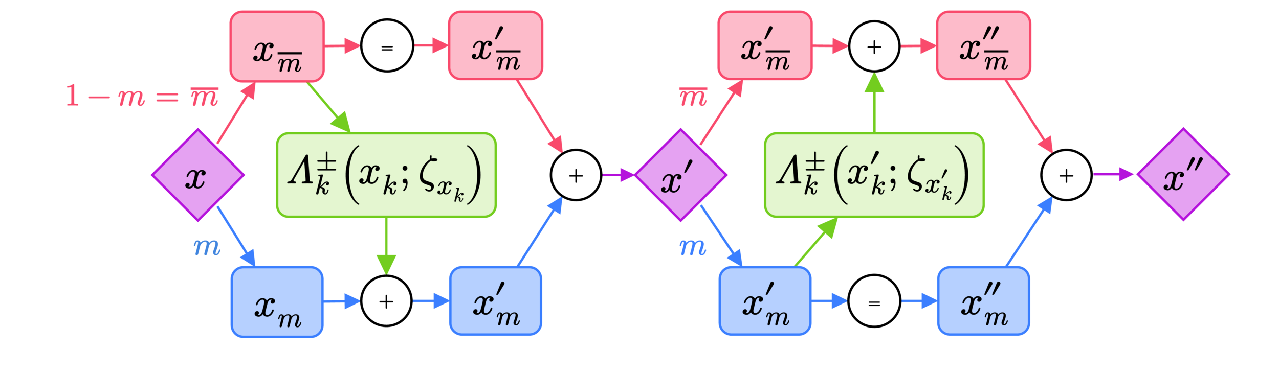
\bar{m}^{t}
m^{t}
=\mathbb{1}
+
Note:
split via \(m^t\)
x^{\prime\prime}_{k} = \hspace{14px}\odot\, \Lambda^{\pm}_{k}(x^{\prime}_{k};\zeta_{x^{\prime}_{k}}) + \hspace{14px}\odot\, x^{\prime}_{k}
\bar{m}^{t}
m^{t}
Network Architecture
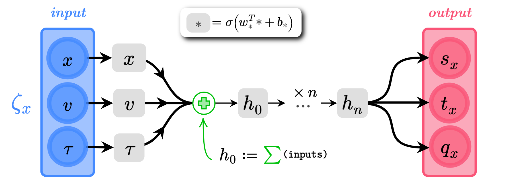
s_{x} = \alpha_{s}\tanh(w^{T}_{s} h_{n} + b_{s})
q_{x} = \alpha_{q}\tanh(w^{T}_{q} h_{n} + b_{q})
t_{x} = w_{t}^{T} h_{n} + b_{t}
(\(\alpha_{s}, \alpha_{q}\) are trainable parameters)
\(x\), \(v\) \(\in \mathbb{R}^{d}\)
\(s_{x}\),\(q_{x}\),\(t_{x}\) \(\in \mathbb{R}^{d}\)
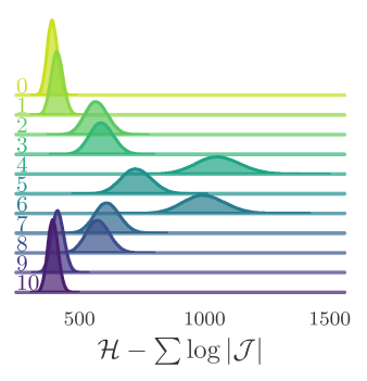
Loss function, \(\mathcal{L}(\theta)\)
- Goal: Maximize "expected squared jump distance" (ESJD), \(A(\xi^{\prime}|\xi)\cdot \delta(\xi^{\prime}, \xi)\):
\ell_{\theta}\left[\xi^{\prime}, \xi, A(\xi^{\prime}|\xi)\right] = \frac{a^{2}}{A(\xi^{\prime}|\xi)\cdot\delta(\xi^{\prime},\xi)} - \frac{A(\xi^{\prime}|\xi)\cdot\delta(\xi^{\prime},\xi)}{a^{2}}
\delta(\xi^{\prime}, \xi) = \|x^{\prime} - x\|^{2}_{2}
- Define the "squared jump distance":
\mathcal{L}_{\theta}\left(\theta\right) \equiv \mathbb{E}_{p(\xi)}\left[\ell_{\theta}\right]
where:
L2HMC
HMC


GMM: Autocorrelation

Annealing Schedule
\left\{\gamma_{t}\right\}_{t=0}^{N} = \left\{\gamma_{0}, \gamma_{1}, \ldots, \gamma_{N-1}, \gamma_{N}\right\},
\gamma_{0} < \gamma_{1} < \ldots < \gamma_{N} \equiv 1
\gamma_{t+1} - \gamma_{t} \ll 1
p_{t}(x)\propto e^{-\gamma_{t}S(x)},\quad\text{for}\quad t=0, 1,\ldots, N
- Introduce an annealing schedule during the training phase:
- For \(\|\gamma_{t}\| < 1\), this helps to rescale (shrink) the energy barriers between isolated modes
- Allows our sampler to explore previously inaccessible regions of the target distribution
- Target distribution becomes:
(varied slowly)
\(= \{0.1, 0.2, \ldots, 0.9, 1.0\}\)
(increasing)
Lattice Gauge Theory
- Link variables:
U_{\mu}(x) = e^{i\varphi_{\mu}(x)} \in U(1)
\varphi_{\mu}(x) \in [-\pi,\pi]
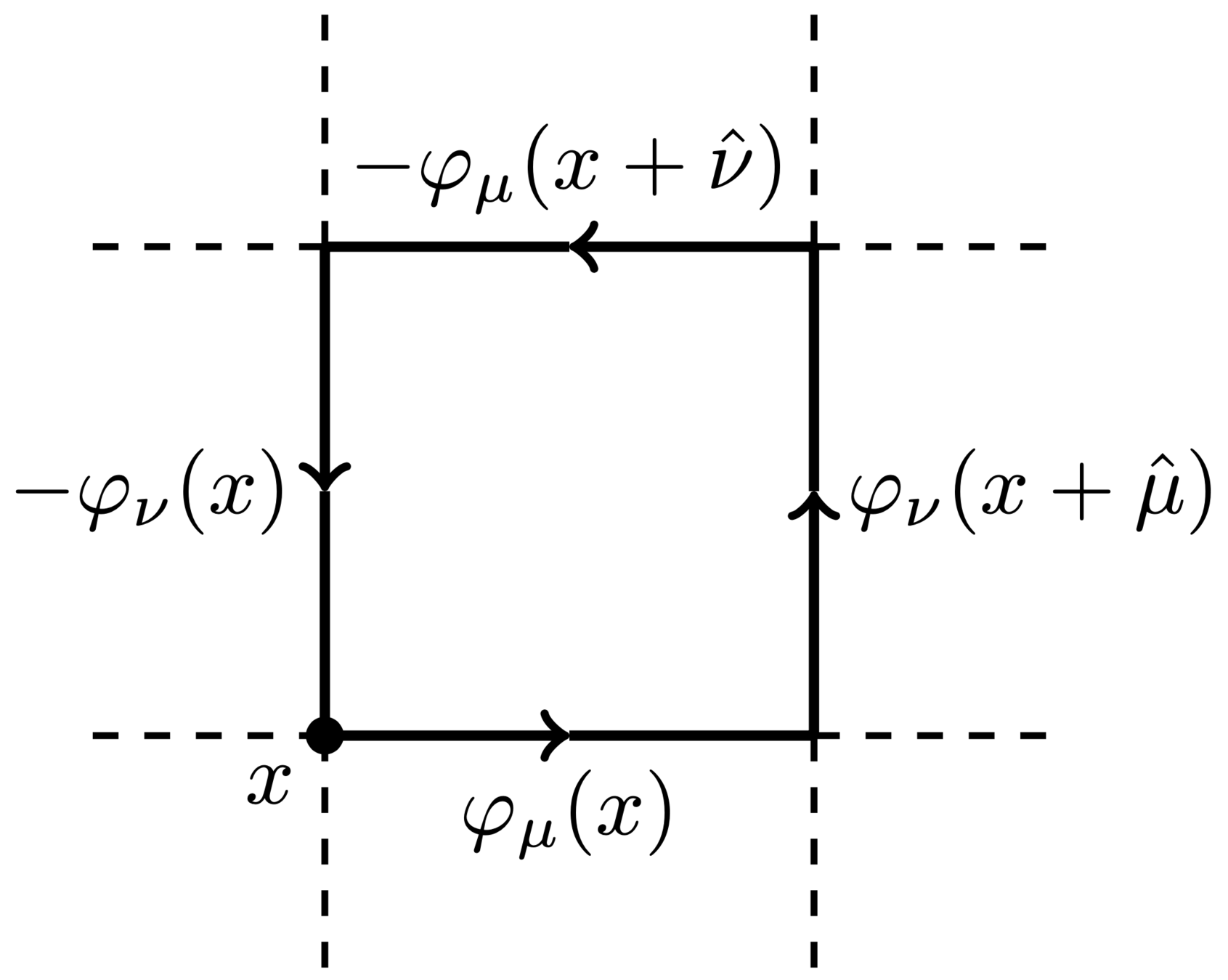
- Wilson action:
S(\varphi)=\sum_{P}1-\cos\varphi_{P}
\varphi_{P} = \varphi_{\mu}(x) + \varphi_{\nu}(x+\hat{\mu}) - \varphi_{\mu}(x+\hat{\nu}) - \varphi_{\nu}(x)
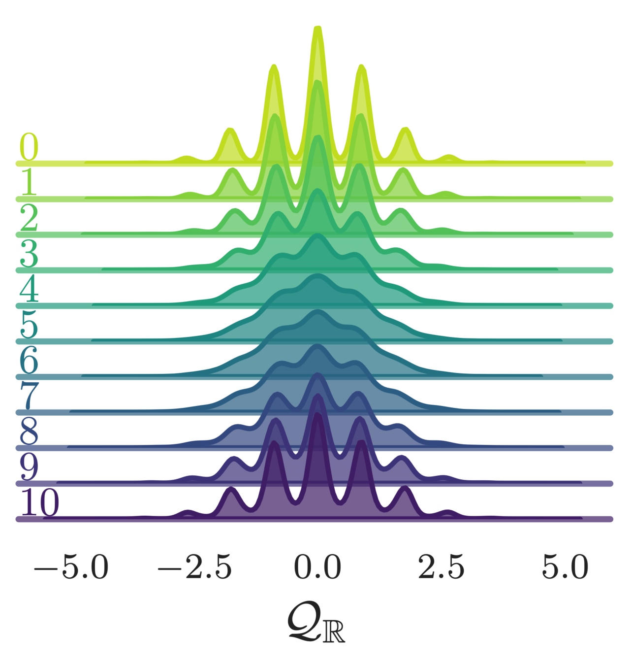
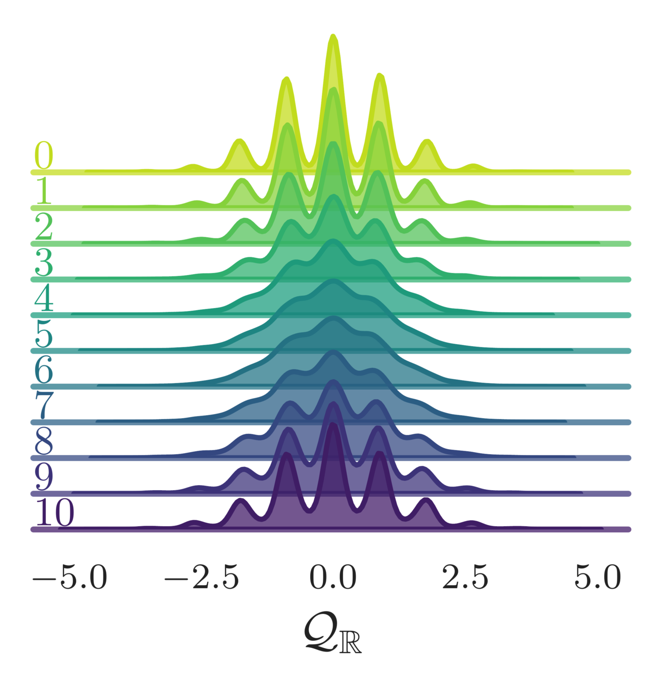
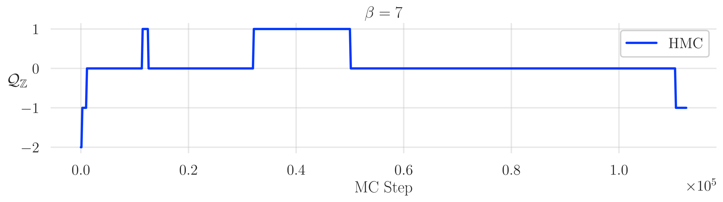
- Topological charge:
\mathcal{Q}_{\mathbb{Z}} = \frac{1}{2\pi}\sum_{P}\left\lfloor\varphi_{P}\right\rfloor \in\mathbb{Z},
\left\lfloor\varphi_{P}\right\rfloor = \varphi_{P} - 2\pi\left\lfloor\frac{\varphi_{P}+\pi}{2\pi}\right\rfloor
\mathcal{Q}_{\mathbb{R}} = \frac{1}{2\pi}\sum_{P}\sin\varphi_{P}\in\mathbb{R}
(real-valued)
(integer-valued)
Lattice Gauge Theory
- Topological Loss Function:
\ell_{\theta}(\xi^{\prime}, \xi, A(\xi^{\prime}|\xi)) = -\frac{1}{a^{2}}A(\xi^{\prime}|\xi)\cdot \delta_{\mathcal{Q}_{\mathbb{R}}}(\xi^{\prime}, \xi)
\delta_{\mathcal{Q}_{\mathbb{R}}}(\xi^{\prime}, \xi) \equiv \left(\mathcal{Q}_{\mathbb{R}}^{\prime} - \mathcal{Q}_{\mathbb{R}}\right)^{2}
= \left(\mathcal{Q}_{\mathbb{R}}(\xi^{\prime}) - \mathcal{Q}_{\mathbb{R}}(\xi)\right)^{2}
\(A(\xi^{\prime}|\xi) = \) "acceptance probability"
where:
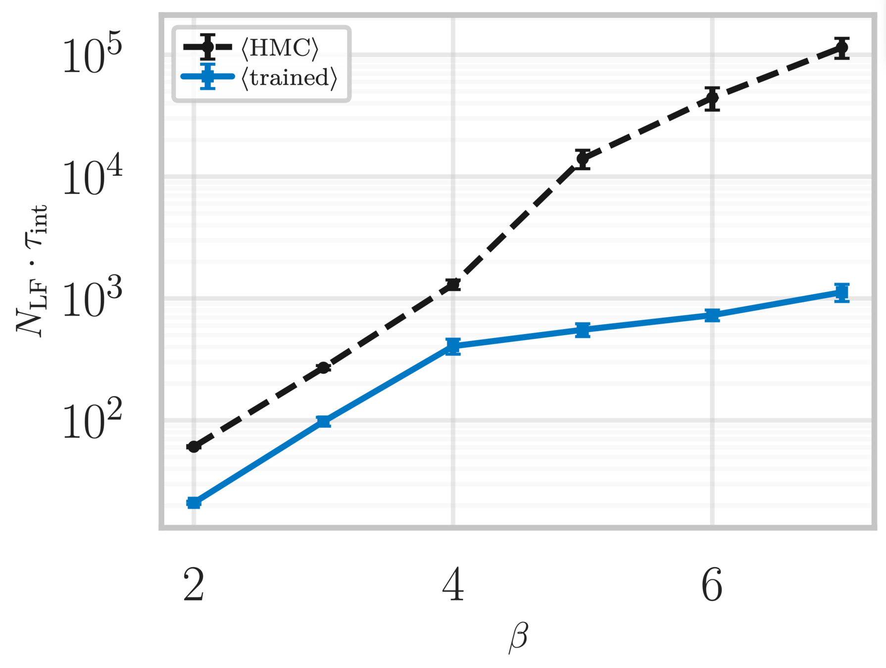
Topological charge history
~ cost / step
continuum limit
Estimate of the Integrated autocorrelation time of \(\mathcal{Q}_{\mathbb{R}}\)
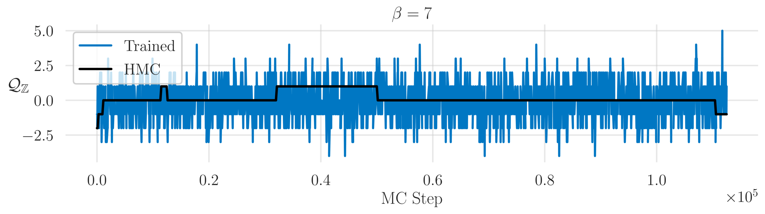
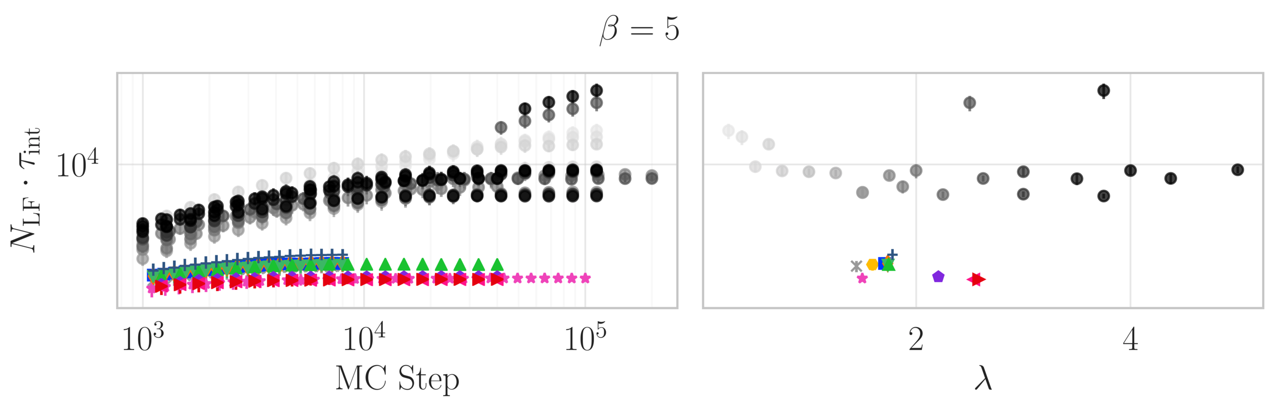
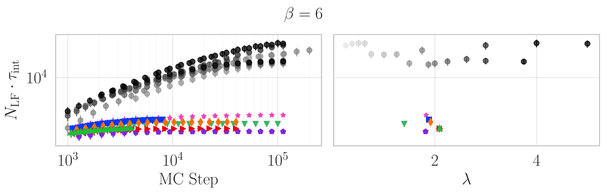
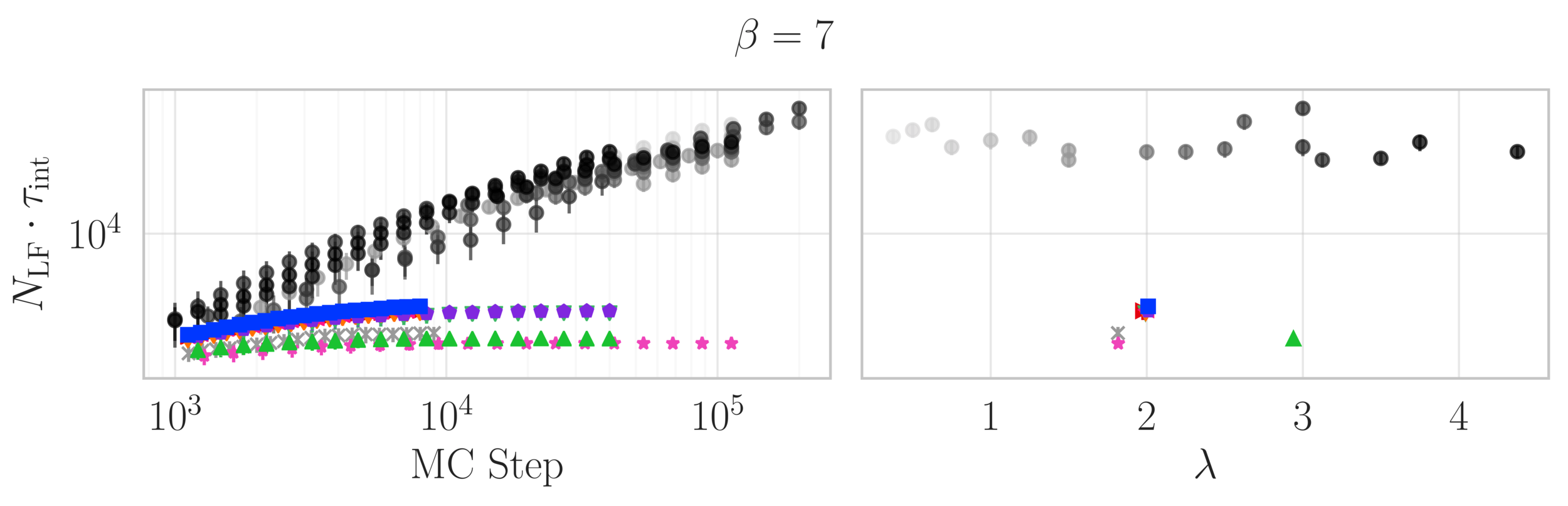
L2HMC
HMC


Lattice Gauge Theory
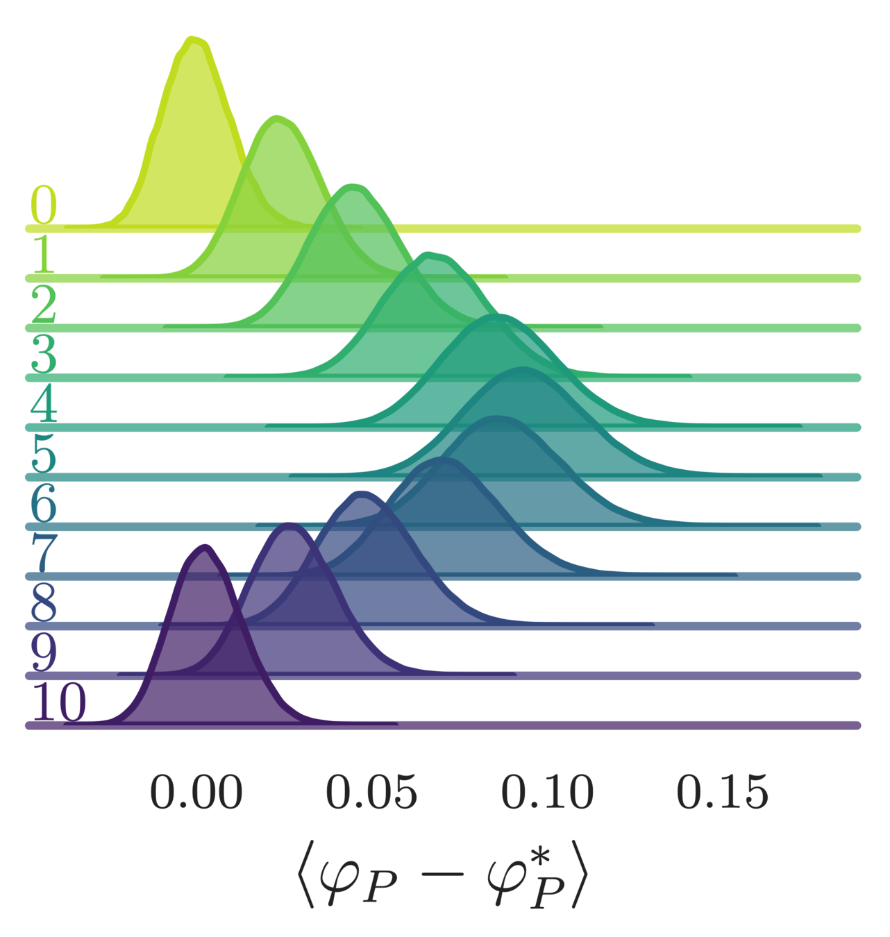
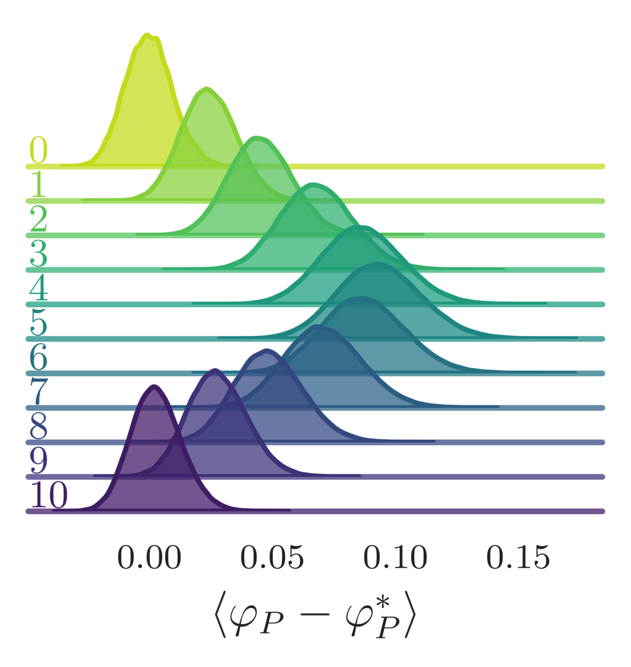
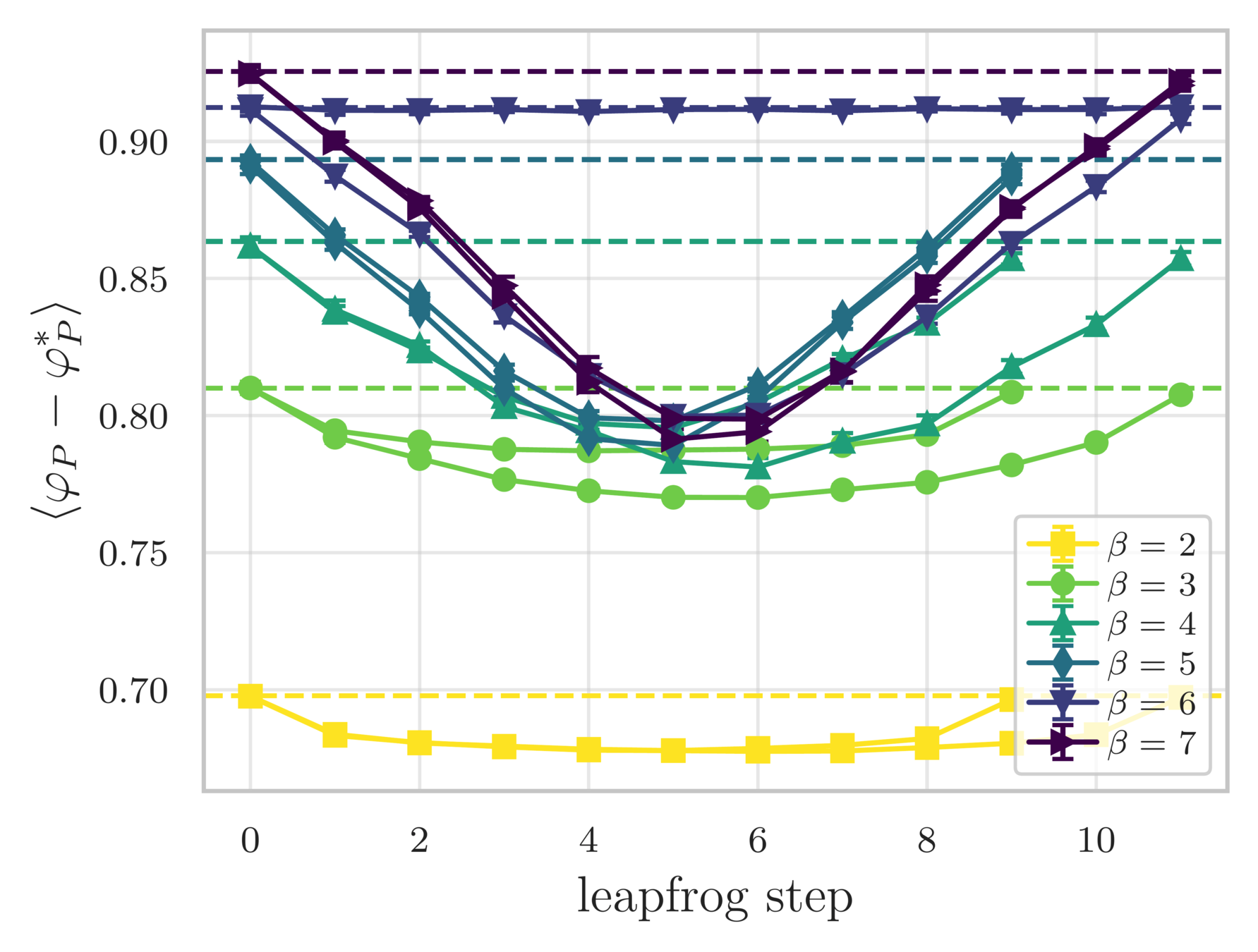
- Error in the average plaquette, \(\langle\varphi_{P}-\varphi^{*}_{P}\rangle\)
- where \(\varphi^{*}_{P} = I_{1}(\beta)/I_{0}(\beta)\) is the exact (\(\infty\)-volume) result

leapfrog step
(MD trajectory)


4096
8192
1024
2048
512
Scaling test: Training
\(4096 \sim 1.73\times\)
\(8192 \sim 2.19\times\)
\(1024 \sim 1.04\times\)
\(2048 \sim 1.29\times\)
\(512\sim 1\times\)

\(4096 \sim 1.73\times\)
\(8192 \sim 2.19\times\)
\(1024 \sim 1.04\times\)
\(2048 \sim 1.29\times\)
\(512\sim 1\times\)
Scaling test: Training
Scaling test: Training


\(8192\sim \times\)
4096
1024
2048
512
Scaling test: Inference
Thanks!
l2hmc-qcd
By Sam Foreman
l2hmc-qcd
L2HMC algorithm applied to simulations in Lattice QCD


