Computational Biology

(BIOSC 1540)

Sep 24, 2024
Lecture 09:
Quantification
Announcements
- A04 is due Friday by 11:59 pm
- Exam is next Thursday (Oct 3rd)


After today, you should be able to
1. Discuss the importance of normalization and quantification in RNA-seq data analysis.
2. Explain the relevance of pseudoalignment instead of read mapping.
3. Understand the purpose of Salmon's generative model.
4. Describe how salmon handles experimental biases in transcriptomics data.
5. Communicate the principles of inference in Salmon.
Let's pause and look at the big picture


Suppose we have isolated a normal and cancerous cell
Cancerous
Normal
We want to identify possible drug targets based on overexpressed genes
We will use transcriptomics!
Defining our transcriptome
Let's simplify our problem to only three transcripts
These represent the only mRNA transcripts we will find in our cells (i.e., the transcriptome)
They have short, medium, and long lengths
Defining our gene expression


We have the following transcript distribution
Normal
Cancerous
More transcripts?
Relative to others?
We have to normalize our transcriptome before making comparisons
2
3
4
We can use transcripts fraction
Ratios are sensitive to total amount


Normal
Cancerous
Because the cancer cell is transcribing more overall, we still get changes across the board
Scaling data to "parts per million"
Real data has more than three transcripts and ratios are substantially smaller (e.g., 0.000001)
This can make computations and communications challenging, so we often scale everything to a million to use unsigned integers
| Transcript | Normal | Cancerous |
|---|---|---|
| 1 | 222,222 | 266,666 |
| 2 | 333,333 | 400,000 |
| 3 | 444,444 | 333,333 |
| Total | 1,000,000 | 1,000,000 |
Small floats require high precision (i.e., float64) and thus memory
Wait, what about sequencing depth?
Longer transcripts will have more reads
Read per kilobase (RPK) corrects this experimental bias through normalization by gene length
(Length is usually just the exons)
RPK example
Reads per kilobase of transcript per million reads mapped
Transcripts per million
After today, you should be able to
1. Discuss the importance of normalization and quantification in RNA-seq data analysis.
2. Explain the relevance of pseudoalignment instead of read mapping.
3. Understand the purpose of Salmon's generative model.
4. Describe how salmon handles experimental biases in transcriptomics data.
5. Communicate the principles of inference in Salmon.
Traditional quantification uses read mapping
Transcriptome
Reads/Fragments
We assign each read to single transcript using our read mapping algorithms
Once aligned, we can count the number of mapped reads to each transcript
1
2
4
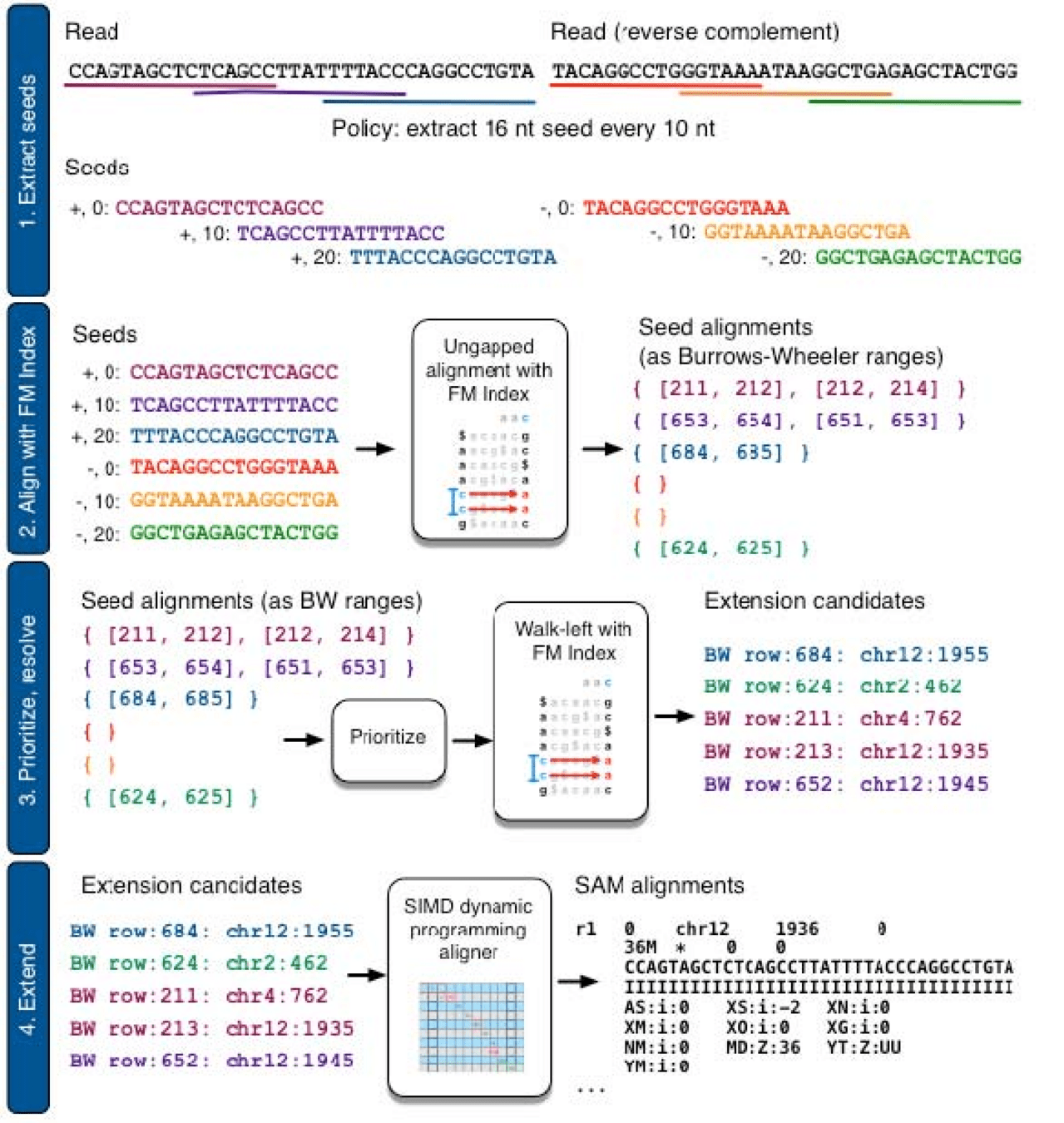
Bowtie 2 uses Burrows-Wheeler Transform to map and quantify reads

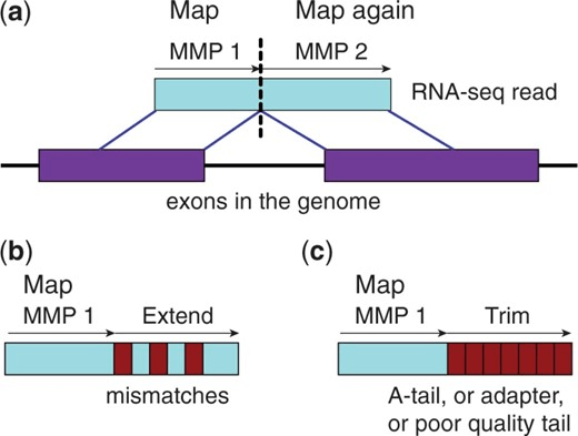
Spliced Transcripts Alignment to a Reference (STAR)

Maximum Mappable Prefix (MMP) approach for fast, accurate spliced alignments
Finds prefix that perfectly matches reference then repeats for unmatched regions
This automatically detects junctions instead of relying on databases
Suppose someone took library books (transcripts) and then shredded them (reads)

In the context of our analogy, we not only need to find the book but which page it was from
This takes a long time
Alignment-based methods need to determine the read's exact position in the transcript
Alignment-based methods are computationally expensive
Identifies which transcripts are compatible with the read, skipping the precise location step
Pseudoalignment finds which transcript, but not where
Analogy: Just find books that are compatible and don't worry about which page

It does not worry about where within that transcript it originated
Alignment
Pseudoalignment
Specifies where exactly in the transcript this read came from
(e.g., at position 478)
Specifies that it came somewhere from this transcript (i.e., compatible)
Pseudoalignment: This method, used by tools like Kallisto, skips the full alignment process. Instead of mapping each read to a specific position, pseudoalignment identifies which transcripts are compatible with a given read
Bypassing alignment accelerates quantification
- Pros: Faster and less resource-intensive than alignment-based methods
- Cons: It may lack certain details, such as the position and orientation of reads, which are useful for correcting technical biases
After today, you should be able to
1. Discuss the importance of normalization and quantification in RNA-seq data analysis.
2. Explain the relevance of pseudoalignment instead of read mapping.
3. Understand the purpose of Salmon's generative model.
4. Describe how salmon handles experimental biases in transcriptomics data.
5. Communicate the principles of inference in Salmon.
Let's understand our problem
Initial sample
We have to use reads to quantity our initial sample
Has some number of transcripts
Fragments
Reads
After PCR amplification and fragmentation
Sequencing with imperfections
What is a generative model?
Generative model: A statistical model that explains how the observed data are generated from the underlying system
Defines a computational framework that produces sequencing reads from a population of transcripts
First, we have to define our model
Salmon's mathematical definition of a transcriptome
Our whole transcriptome
Individual transcripts
Transcript counts
Salmon's formulation of transcript abundance
So far, we have been talking about transcript fractions
We can also take nucleotide fractions by taking into account the effective length of each transcript
This tells us how much of the total RNA pool comes from each transcript
I will explain the effective length later. For now, think of it as a "corrected" length
Converting to relative abundances
The transcript fraction tells us the proportion of total RNA molecules in the sample that come from transcript i
This gives the relative abundance of each transcript i
Adjusts for the fact that longer transcripts generate more reads
The transcript fraction normalizes nucleotide fraction by the effective length
TPM is "Transcripts per million"
Transcript-Fragment Assignment Matrix
is a binary matrix (i.e., all values are 0 or 1)
of M transcripts (rows) and N fragments (columns)
if fragment j is assigned to transcript i
Transcript 1
Transcript 2
Transcript M
...
Fragment 1
Fragment 2
Fragment N
...
Z example
Suppose we have 3 transcripts and 12 fragments
Z is just how we computationally assign fragments to transcripts
Generative model inference
Transcript-fragment assignment
Transcript abundance
N and M are same as experiment
Given these inputs, generate a distribution of fragments
Run 1
Run 2
Known from organism and experiment
Probability of observing the sequence fragments
Which scenario is more likely, given our generative model?
We can use probabilistic methods to find parameters that explain our observed distirbution
Conditional probability notation
This reads, "What is the probability of a occurring if b is true?"

Given this Radar, what is the probability of Rain in Oakland?
=
Example
Probability of observing the sequenced fragments
Given these parameters, how probable is it that our experiment generated these observed reads?
Optimize these values until we get the highest probability
Available transcripts
Transcript-fragment assignment
Transcript abundance
After today, you should be able to
1. Discuss the importance of normalization and quantification in RNA-seq data analysis.
2. Explain the relevance of pseudoalignment instead of read mapping.
3. Understand the purpose of Salmon's generative model.
4. Describe how salmon handles experimental biases in transcriptomics data.
5. Communicate the principles of inference in Salmon.
Probability of observing the sequenced fragments
We can now compute the probability of observing:
Set of fragments
Given:
Transcript assignment
Transcript abundance
Probability of observing fragment
given that it comes from transcript
This expression accounts for all possible transcripts a fragment might come from, weighted by how likely that fragment is to come from each transcript
Transcriptome
Fragment probabilities
is a conditional probability that depends on the position of the fragment within the transcript, the length of the fragment, and any technical biases
In Salmon’s quasi-mapping approach, this probability is approximated based on transcript compatibility rather than exact positions.
Positional bias
A transcript’s effective length adjusts for the fact that fragments near the ends of a transcript are less likely to be sampled
Fragments from central regions are more likely to be of optimal length for sequencing reads
Fragments that include transcript ends might be too short
Mean of the truncated empirical fragment length distribution
After today, you should be able to
1. Discuss the importance of normalization and quantification in RNA-seq data analysis.
2. Explain the relevance of pseudoalignment instead of read mapping.
3. Understand the purpose of Salmon's generative model.
4. Describe how salmon handles experimental biases in transcriptomics data.
5. Communicate the principles of inference in Salmon.
Introduction to inference in Salmon
-
Inference refers to the process of estimating transcript abundances from observed RNA-seq reads using statistical models.
- Salmon’s inference process involves estimating the most likely abundance of each transcript that could explain the observed set of fragments (reads).
- It does this by solving a complex, high-dimensional problem where each fragment might map to multiple transcripts.
Two-phase inference in salmon
This two-phase approach balances speed (in the online phase) with accuracy (in the offline phase)
Salmon processes reads in two stages
Online phase
Makes fast, initial estimates of transcript abundances as the reads are processed
Offline phase
Refines these initial estimates using more complex optimization techniques
Online phase:
Stochastic variational inference
Initial estimates using quasi-mapping
Quasi-mapping is A fast, lightweight technique used to associate RNA-seq fragments with possible transcripts
Alignment is expensive, so quasi-mapping stops after identify seeds
Essentially early stopping of read mapping
Read mapping
GAT
[7, 14]
h(k)
CCGTATCGATTGCAGATG
Identify seeds, then extend and compute base-by-base alignment
This is what initializes compatible transcripts and abundance
Iteratively update parameters based on mini batches
Mini-batch 1
Mini-batch 2
Mini-batch 3
Take current parameters
Compute derivatives from batch
Update parameters (i.e., abundances)
Repeat for each batch
Offline Phase:
Expectation-Maximization (EM) algorithm
After the online phase, Salmon refines the estimates using a more complex optimization method, typically based on the Expectation-Maximization (EM) algorithm
Offline phase fine tunes transcript abundance
This phase ensures the accuracy of abundance estimates, incorporating the bias corrections learned during the online phase
Likelihood of the Data
This is the probability of observing the entire set of fragments FFF, given the transcriptome TTT and nucleotide fractions η\etaη
The goal is to maximize this likelihood to infer the most likely values of η\etaη, which correspond to the relative abundances of the transcripts
The likelihood function is central to the inference process in Salmon:
Optimize the estimates of α, a vector of the estimated number of reads originating from each transcript
Maximum Likelihood Estimation (MLE)
The goal of maximum likelihood is to find the parameters (transcript abundances) that maximize the probability of the observed data (sequenced reads)
Optimize the estimates of α, a vector of the estimated number of reads originating from each transcript
Given α, η can be directly computed.
The likelihood function is central to the inference process in Salmon:
Why the EM Algorithm Maximizes the Likelihood
The EM algorithm works by breaking down a difficult problem into two simpler problems:
- In the E-step, we estimate the missing information (the assignment of fragments to transcripts) using the current transcript abundance estimates.
- In the M-step, we use the estimated assignments to update the transcript abundances, improving the likelihood.
At each iteration, the likelihood of the observed data increases, and the EM algorithm iteratively refines the transcript abundance estimates until it reaches a maximum
Before the next class, you should
Lecture 10:
Differential gene expression
Lecture 09:
Quantification
Today
Thursday
Learning bias parameters
For the first 5,000,000 observations we learn these defined bias parameters
Probability of generating fragment j from transcript i
Probability of drawing a fragment of the inferred length given t
Probability of fragment starting at position p on t
Probability of obtaining a fragment with the given orientation
Probability of alignment of fragment j given these mapping and transcript conditions
Probability of alignment fragment to transcript
Represents the probability of the alignment starting at a particular position or state sos_o
The probability of the fragment "transitioning to another state"
Essentially, how likely does this fragment align somewhere else
For fun: Hidden Markov Models
BIOSC 1540: L09 (Quantification)
By aalexmmaldonado
BIOSC 1540: L09 (Quantification)
- 100


