
Computational Biology

(BIOSC 1540)

Sep 26, 2024
Lecture 10:
Differential gene expression


Announcements

After today, you should be able to
Why are we learning about differential gene expression?
What is Differential Gene Expression?
Differential Gene Expression (DGE): The process of identifying and quantifying changes in gene expression levels between different sample groups or conditions
- Sample Collection: Gather samples from different conditions (e.g., healthy vs. diseased).
- RNA Sequencing (RNA-seq): Quantify gene expression levels using high-throughput sequencing technologies.
- Read Mapping and Quantification: Align RNA-seq reads to a reference genome and quantify expression (e.g., using Salmon).
- Statistical Analysis: Identify genes with significant expression differences between conditions.
Case study: Breast cancer
-
Objective: Identify genes differentially expressed between triple-negative breast cancer (TNBC) and hormone receptor-positive breast cancer
-
Findings:
- TNBC shows upregulation of genes involved in cell proliferation and metastasis.
-
Implications:
- Targets for specific therapies.
- Improved classification and prognosis of breast cancer subtypes.
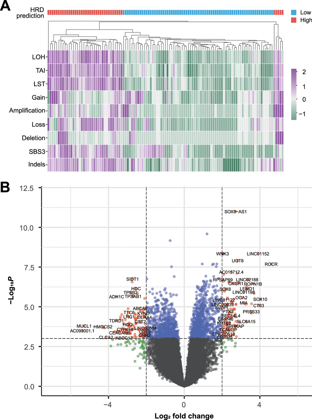
Differential gene expression provides statistical tools to identify changes between samples
After today, you should be able to
Explain the purpose of statistical models and hypothesis testing
What is a statistical model?
A statistical model is a mathematical tool that describes how data are generated
Gene expression
Normal
Cancerous
- Is there an apparent difference in gene expression between the two conditions?
- If so, is it real, or could it have happened by random chance or experimental flaws?
It helps us answer:
Statistical models help us make sense of complex data by identifying patterns and determining whether differences are meaningful or just due to chance
Hypothesis testing in RNA-seq data
After fitting a statistical model, we need to perform hypothesis testing to see if the difference in expression between conditions is statistically significant
Null Hypothesis (H₀): There is no difference in gene expression between the two conditions
Gene expression
Normal
Cancerous
Alternative Hypothesis (H₁): There is a significant difference in gene expression between the conditions
We have two hypotheses:
We reject the null hypothesis when our statistical test demonstrates that the observed difference, if any, is unlikely to have happened by random chance
The P-value is the probability of the null hypothesis being true
What is the probability that any difference is either (1) nonexistent or (2) due to random chance (i.e., "getting lucky")
Probability value (p-value):
The higher the p-value, the more our model supports the null hypothesis
The lower the p-value, the more our model supports the alternative hypothesis
Gene expression
Normal
Cancerous
Gene expression
Normal
Cancerous
Differential gene expression uses statistical models for hypothesis testing
Ensures that we are not biasing our data or our interpretation
After today, you should be able to
Discuss the challenges of working with gene expression data
The nature of count data
RNA-seq generates count data – the number of RNA fragments that map to each gene
Gene expression
Normal
Cancerous
Example: 573,282 TPM
Discrete data requires us to use special statistical tools
- Data that can only take specific values (like whole numbers)
- In RNA-seq, we measure the number of reads mapped to a gene, so the data are count-based
- You can't have "half a read" or a decimal number of reads.
What is discrete data:
For example, you cannot use a normal distribution because it requires continuous data
Binomial: A Simple Model for Discrete Counts
The Binomial distribution models the number of successes in a fixed number of independent trials, where each trial has the same probability of success
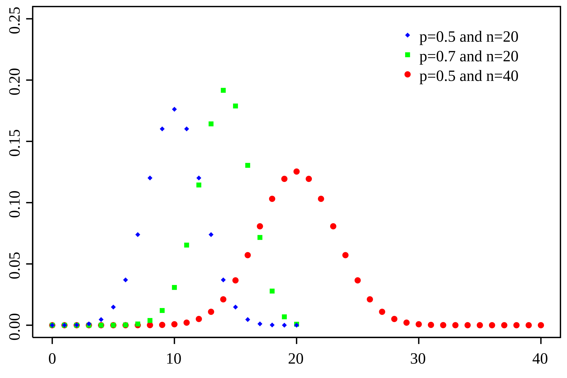
Number of trials
Number of successes
Probability
Probability of success
RNA-seq analogy: Each read can be considered a "trial," and the probability that a read maps to a specific gene is the "probability of success."
Limitations of Binomial distributions for RNA-Seq
- Main limitation: Assumes that the probability of success is constant between samples
- Smaller limitation 1: The number of possible trials can be very large, especially when sequencing at a high depth
- Smaller limitation 2: The probability of expression is very small for many genes because they are either lowly expressed or not at all
The Poisson distribution simplifies computation and allows for varying probabilities
Computations with low p and high n are computationally demanding
Poisson distribution: A baseline for modeling discrete counts
The Poisson distribution is a statistical tool used to model the number of events (or counts) that happen in a fixed period of time or space, where:
- The events are independent of each other
- Each event has a constant average rate
Expected average of X
Number of events or counts
Probability
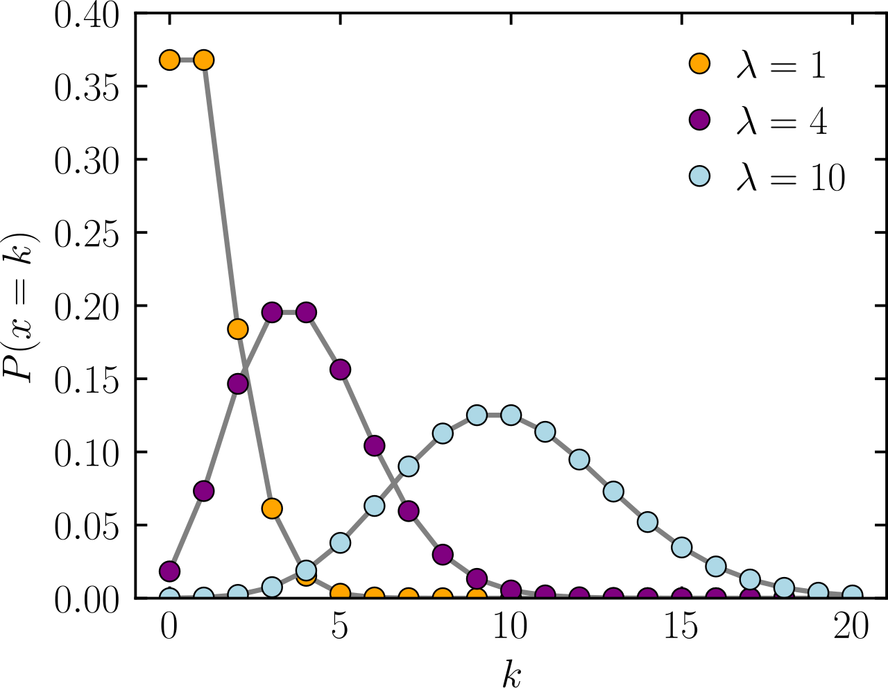
Provides an accurate distribution of counts if your mean and variance are approximately equal
Poisson distribution becomes inaccurate when variance > mean


RNA-seq data are noisy (i.e., high variance) and incompatible with Poisson distribution
Parity plots with mean and variance show deviations with Poisson distributions
Higher counts typically have a larger variance
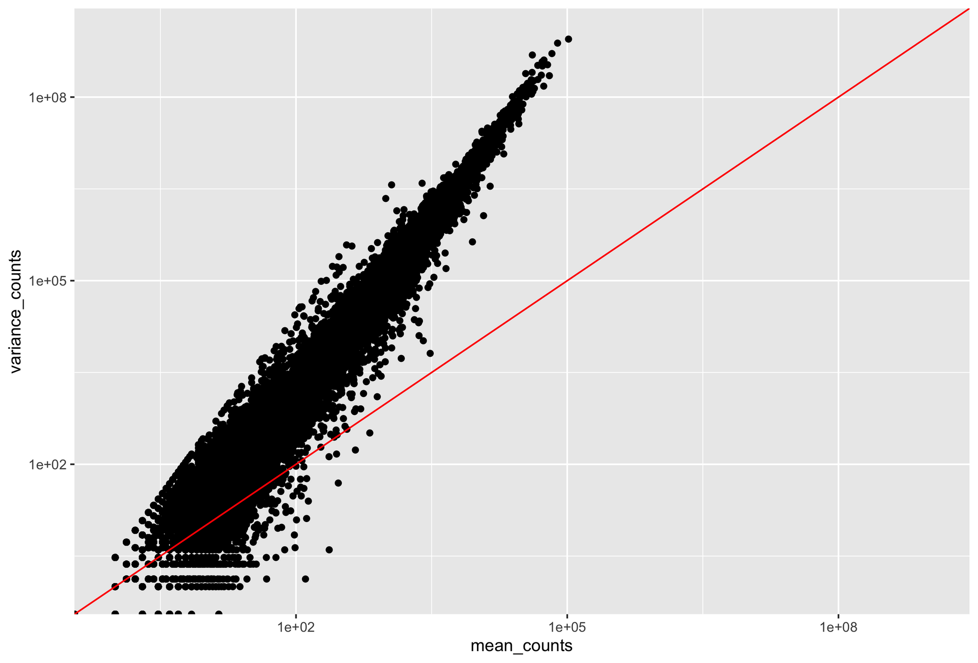
Count mean
Count variance
Mean = variance line
Overdispersion in RNA-Seq
Overdispersion: It happens when the variance in the data is larger than what is predicted by simpler models (e.g., Poisson distribution)
- Expected variance for Poisson-distributed data equals the mean: Variance=μ\text{Variance} = \muVariance=μ
- Variance is often larger than the mean for RNA-Seq: Variance>μ\text{Variance} > \muVariance>μ

Overdispersion may reflect biological variability between samples not captured by the experimental conditions
- Differences in RNA quality
- sequencing depth,
- biological factors like different cell types within the same tissue
Negative Binomial distribution accounts for high dispersion
Observed number of counts
Mean or expected value of counts
Dispersion parameter, controlling how much the variance exceeds the mean
Gamma function, which generalizes the factorial to floats
If α=0\alpha = 0α=0, the Negative Binomial distribution reduces to the Poisson distribution
The Challenge of zeros in RNA-seq data
RNA-seq data frequently contains zero counts for some genes because not all genes are expressed under all conditions
Most statistical models account for variance, but not that zeros can dominate counts
For example, if we have a high expected mean with Poisson distribution we can still have zeros or very low counts

In these circumstances, we have to use zero-inflated models
We will ignore these for now
After today, you should be able to
Discuss fitting of statistical models
Why are statistical models important in RNA-seq?
RNA-seq data is messy: counts vary, there are lots of zeros, and data doesn’t follow simple patterns
- Step 1: The model looks at the data from both groups
- Step 2: It considers how much variation there is within each group
- Step 3: The model calculates how likely it is to see the average difference if there is no real difference between the groups (just by chance)
We need models to account for this complexity and figure out which genes are differentially expressed in a meaningful way
Define the model for each gene
A statistical model predicts each sample's count data
(number of reads mapping to each gene)
- It accounts for the mean (average expression for a gene) and the dispersion (how much the expression varies across samples)

Fit parameters using optimization algorithms
MLE tries to find the model parameters that make the observed counts most likely

- We use maximum likelihood estimation (MLE) to estimate the parameters μ\muμ (mean) and α\alphaα (dispersion) for each gene.
- MLE finds the values of the parameters that maximize the likelihood of observing the data given the model.
It does this by adjusting the model until the predicted counts match the actual counts as closely as possible (i.e., minimize the error)
After today, you should be able to
Understand statistical tests used for gene expression data
Wald’s Test for Gene Expression Differences
-
Wald’s Test: A statistical test that helps us determine whether the estimated log fold change between two conditions is significantly different from zero.
-
Null Hypothesis (H₀): The log fold change between conditions is zero (no difference in expression between the conditions).
- Log Fold Change (β₁) = 0 means that the gene is expressed at the same level in both conditions.
-
Alternative Hypothesis (H₁): The log fold change between conditions is not zero (there is a difference in expression).
Log Fold Change
- Positive Log Fold Change: Indicates higher expression in the condition of interest (e.g., diseased).
- Negative Log Fold Change: Indicates lower expression in the condition of interest.
- Log Fold Change of Zero: Means no difference between conditions.
Estimate Parameters from the Negative Binomial Model
For each gene, the Negative Binomial model gives us an estimated log fold changeβ^1\hat{\beta}_1
It also gives us a standard error (SE) for this estimate, which tells us how uncertain we are about the estimate of log fold changeβ^1\hat{\beta}_
The Wald statistic is calculated as
This statistic tells us how many standard deviations the estimated log fold change is away from zero (no difference)
Likelihood Ratio Test
To compute a p-value, a likelihood ratio test (LRT) can be usedβ^1\hat{\beta}_1
The idea is to compare the likelihood of the data under
- the null model (same expression in both conditions)
- the alternative model (different expression levels in each condition)β^1\hat{\beta}_1
Log-Likelihood of Negative Binomial
For each condition, you compute the log-likelihoods:
LRT Statistic
The LRT statistic is:β^1\hat{\beta}_1
The log-likelihood under the null hypothesis (assuming a common mean μ0\mu_0μ0 for both conditions)
The LRT statistic approximately follows a chi-squared distribution with 1 degree of freedom under the null hypothesis
The p-value is computed as:
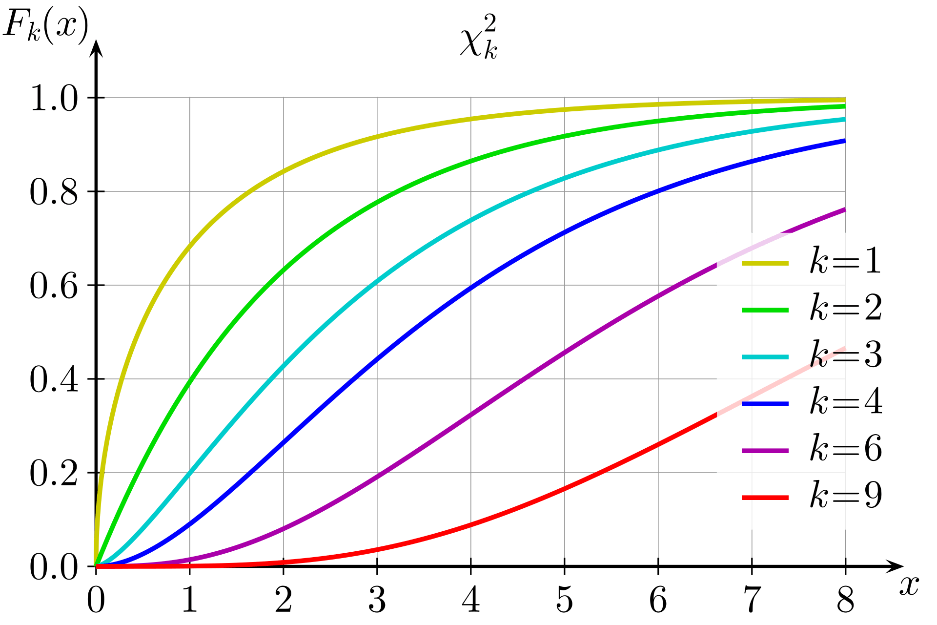
k would be 1
After today, you should be able to
Interpret common visualizations used in differential expression analysis
Visualizing Significance vs. Magnitude of Expression Changes
Interpretation:
- Top Corners: Genes with high significance and large fold changes (both upregulated and downregulated)
- Center: Genes with little to no change or low significance

A volcano plot displays the relationship between each gene's statistical significance (p-value) and the magnitude of change (fold change).
MA Plots
An MA plot visualizes the relationship between the average expression (A) and the log fold change (M) for each gene.

Interpretation:
- Center Line (M=0): No change in expression
- Spread: Indicates variability in fold changes across different expression levels
Usage: Identifying trends or biases in expression data, such as mean-dependent variance.
Heatmaps
Components:
- Rows: Genes
- Columns: Samples
- Color Intensity: Represents expression level (e.g., red for upregulation, blue for downregulation)

A heatmap displays the expression levels of multiple genes across different samples using color gradients
Interpretation: Identifying clusters of co-expressed genes and sample groupings based on expression profiles.
Principal Component Analysis (PCA) Plots
PCA transforms high-dimensional gene expression data into principal components that capture the most variance

Axes: Principal components representing the most significant sources of variation
Interpretation:
- Sample Clustering: Samples from similar conditions cluster together.
- Outliers: Samples that do not group with others may indicate technical or biological variability.
Usage: Assessing batch effects, overall data structure, and sample quality
Before the next class, you should
- Turn in A04
- Study for exam
- Treat yourself
Review
Lecture 10:
Differential gene expression
Today
Tuesday
BIOSC 1540: L10 (Differential gene expression)
By aalexmmaldonado
BIOSC 1540: L10 (Differential gene expression)
- 71


