Introduction to
Normalizing Flows
Justine Zeghal
Lecture at the 2023 AstroInformatics school in Fréjus


Content
- Motivations
- Generative Models
- Normalizing Flows
- Different architectures
Motivations
Quick probability recap
\text{Density function:
}
\text{Let $X$ be a continuous random variable.}\\
\text{The probability distribution or probability density function}\\
\text{of $X$ is a function $p(x)$ such that
}
\mathbb{P}(a \leq X \leq b) = \int_a^b p(x)dx, \text{with $a \leq b$.}
p(x)
p(x) \geq 0 \text{ for all } x
\int_{-\infty}^{+\infty} p(x) dx = 1
Why do we care?
p(x)
X
hmmm ok 🤨 but why?
Classical / old methods
Classical / old methods
\text{
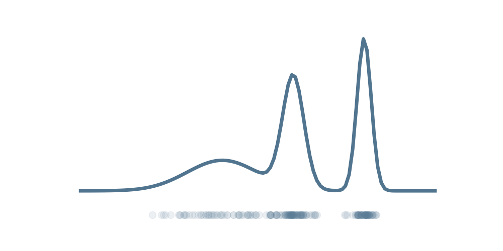
Kernel Density Estimation (KDE):
}
Classical / old methods
\text{
Kernel Density Estimation (KDE):
}
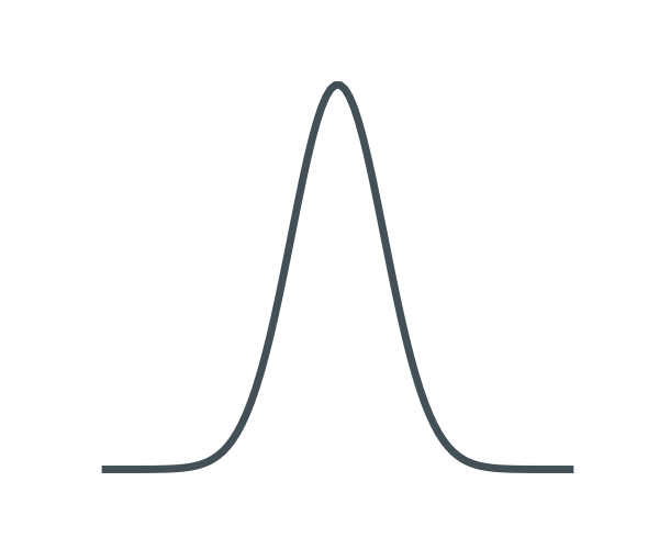
\text{
KDE is a non-parametric method }\\
\text{that estimates the density by} \\
\text{placing a kernel (e.g., Gaussian)}\\
\text{at each data point and summing}\\
\text{them up to create a smooth density }\\
\text{function.}
Classical / old methods
\text{
Kernel Density Estimation (KDE):
}
\text{
KDE is a non-parametric method }\\
\text{that estimates the density by} \\
\text{placing a kernel (e.g., Gaussian)}\\
\text{at each data point and summing}\\
\text{them up to create a smooth density }\\
\text{function.}
Classical / old methods
\text{
Kernel Density Estimation (KDE):
}
\text{
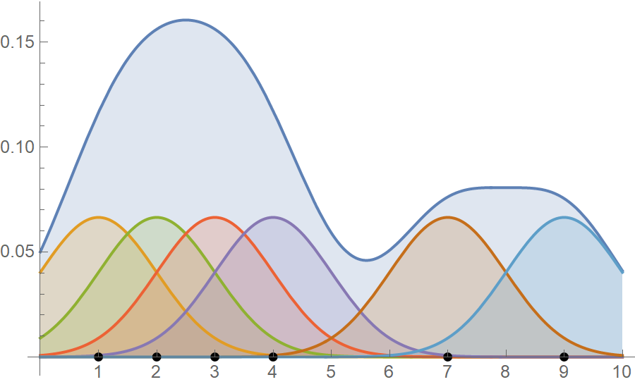
Gaussian Mixture Models (GMM):
}
\text{
KDE is a non-parametric method }\\
\text{that estimates the density by} \\
\text{placing a kernel (e.g., Gaussian)}\\
\text{at each data point and summing}\\
\text{them up to create a smooth density }\\
\text{function.}
Classical / old methods
\text{
Kernel Density Estimation (KDE):
}
\text{
Gaussian Mixture Models (GMM):
}
\text{
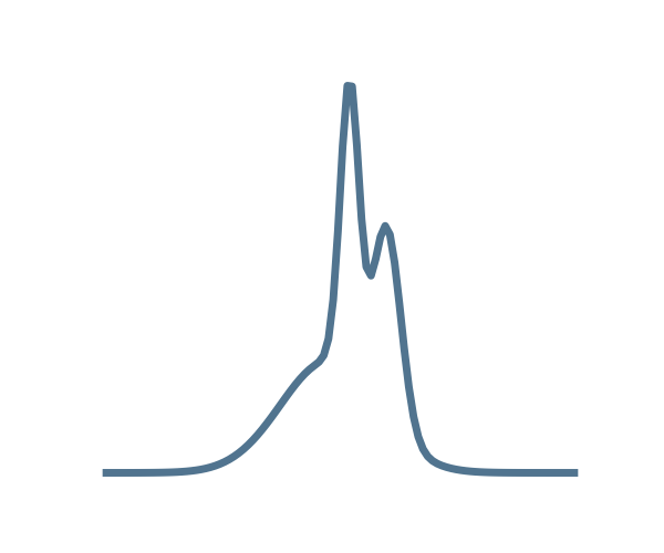
GMM approximate the density as a weighted sum of Gaussian}\\
\text{distributions. The parameters (mean, covariance, and weights)}\\
\text{are estimated by maximizing the likelihood.
}
\text{
KDE is a non-parametric method }\\
\text{that estimates the density by} \\
\text{placing a kernel (e.g., Gaussian)}\\
\text{at each data point and summing}\\
\text{them up to create a smooth density }\\
\text{function.}
Classical / old methods
\text{
Kernel Density Estimation (KDE):
}
\text{
Gaussian Mixture Models (GMM):
}
\text{
GMM approximate the density as a weighted sum of Gaussian}\\
\text{distributions. The parameters (mean, covariance, and weights)}\\
\text{are estimated by maximizing the likelihood.
}
\text{
KDE is a non-parametric method }\\
\text{that estimates the density by} \\
\text{placing a kernel (e.g., Gaussian)}\\
\text{at each data point and summing}\\
\text{them up to create a smooth density }\\
\text{function.}
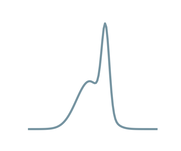
\text{Flexibility in modeling complex distributions.}\\
\text{Data generation capabilities.}\\
\text{Scalability with dimension.}
Classical / old methods
\text{
Kernel Density Estimation (KDE):
}
\text{
Gaussian Mixture Models (GMM):
}
\text{
GMM approximate the density as a weighted sum of Gaussian}\\
\text{distributions. The parameters (mean, covariance, and weights)}\\
\text{are estimated by maximizing the likelihood.
}
\text{
KDE is a non-parametric method }\\
\text{that estimates the density by} \\
\text{placing a kernel (e.g., Gaussian)}\\
\text{at each data point and summing}\\
\text{them up to create a smooth density }\\
\text{function.}
\text{Flexibility in modeling complex distributions.}\\
\text{Data generation capabilities.}\\
\text{Scalability with dimension.}
\text{$\implies$ need for new methods }
Generative Models
What is generative modeling?
\text{Or how to undestrand the world from data?}
😎
What is generative modeling?
\text{Or how to undestrand the world from data?}
😎
\text{The goal of generative modeling is to capture the complex patterns}\\
\text{and structures embedded in the data by learning the underlying} \\
\text{probability distribution.}
What is generative modeling?
\text{Or how to undestrand the world from data?}
😎
\text{The goal of generative modeling is to capture the complex patterns}\\
\text{and structures embedded in the data by learning the underlying} \\
\text{probability distribution.}
\text{Given a set of data $X = \{X_1, X_2, ..... X_N\}$ our goal is to }\\
\text{re construct the generation process that gave rise to this dataset.}
\text{This means building a parametric model $p_{\phi}$ that tries to be close to $p$.}

\text{True distribution } p(x)
\text{Sample } x \sim p(x)
\text{Model } p_{\phi}(x)

What is generative modeling?
\text{Or how to undestrand the world from data?}
😎
\text{The goal of generative modeling is to capture the complex patterns}\\
\text{and structures embedded in the data by learning the underlying} \\
\text{probability distribution.}
\text{Given a set of data $X = \{X_1, X_2, ..... X_N\}$ our goal is to }\\
\text{re construct the generation process that gave rise to this dataset.}
\text{This means building a parametric model $p_{\phi}$ that tries to be close to $p$.}
\text{True distribution } p(x)
\text{Sample } x \sim p(x)
\text{Model } p_{\phi}(x)

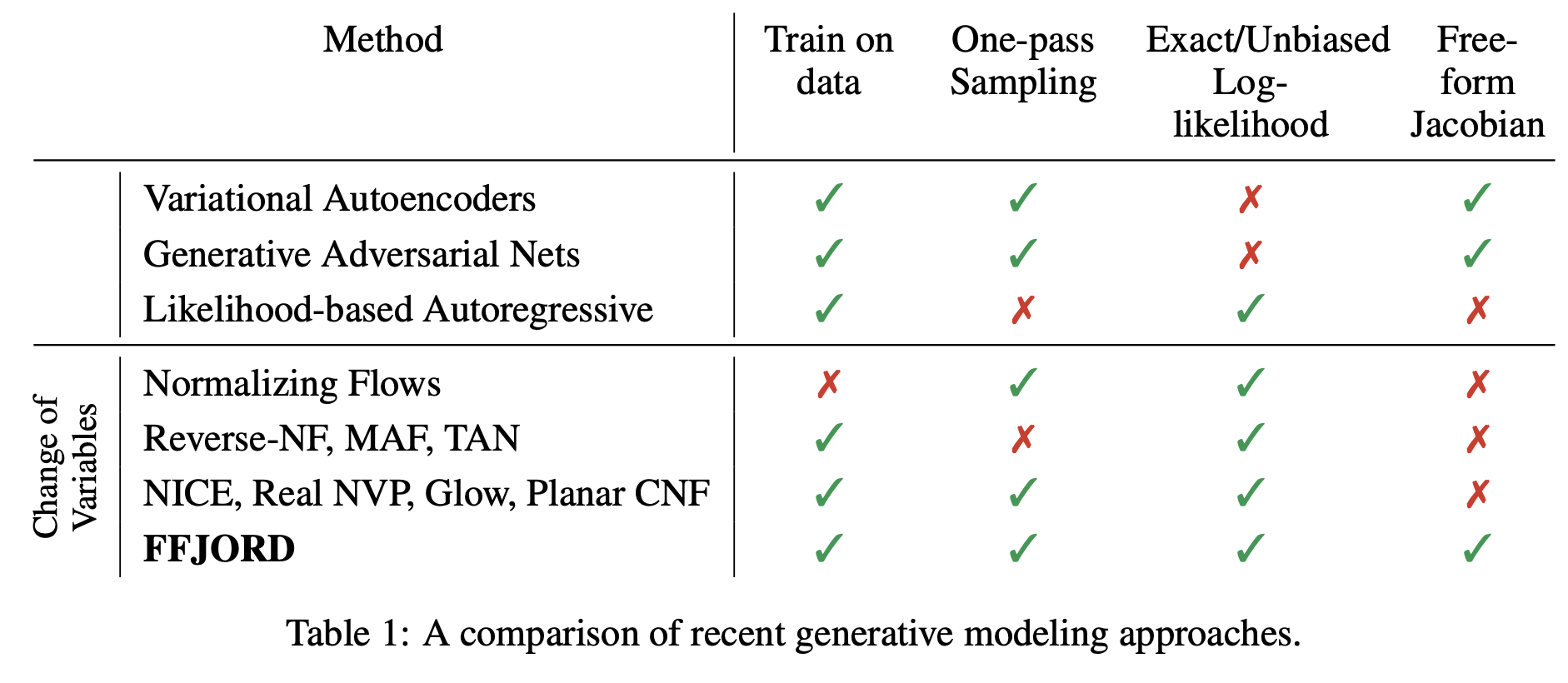
Comparison of generative modeling approaches
reference: https://arxiv.org/pdf/1810.01367.pdf
Comparison of generative modeling approaches
reference: https://arxiv.org/pdf/1810.01367.pdf
Comparison of generative modeling approaches
reference: https://arxiv.org/pdf/1810.01367.pdf
Normalizing Flows
reference: https://arxiv.org/abs/1906.12320
reference: https://blog.evjang.com/2019/07/nf-jax.html
Basic idea
p_x(x)
p_z(z)
f(z)
\text{Normalizing Flows (NF) are based on mapping functions $f : \mathbb{R}^n \to \mathbb{R}^n$.} \\
\text{Those functions enable us to map a latent variable} \\
\text{$z \sim p_z(z)$ to a variable $x \sim p_x(x)$.}
\text{Approximating distributions through the use of NF is ONLY}\\
\text{a matter of learning this mapping function $f : \mathbb{R}^n \to \mathbb{R}^n$.}
p_x(x)
p_z(z)
Bijection
p_x(x)
p_z(z)
Bijection
f(z)
p_x(x)
p_z(z)
Bijection
f(z)
p_x(x)
p_z(z)
Bijection
\text{sampling}
f(z)
p_x(x)
p_z(z)
Bijection
p_x(x)
p_z(z)
Bijection
p_x(x)
p_z(z)
Bijection
f^{-1}(x)
p_x(x)
p_z(z)
Bijection
f^{-1}(x)
p_x(x)
p_z(z)
Bijection
\text{evaluation}
f^{-1}(x)
p_x(x)
p_z(z)
Bijection
Bijection
f(z)
f^{-1}(x)
p_x(x)
p_z(z)
Bijection
f(z)
f^{-1}(x)
p_x(x)
p_z(z)
\text{The mapping $f$ between $z$ and $x$ has to be an invertible function.}
Bijection
\text{The mapping $f$ between $z$ and $x$ has to be an invertible function.}
f(z)
f^{-1}(x)
p_x(x)
p_z(z)
reference: fr.wikipedia.org/wiki/Bijection

z
z
z
x
x
x
Bijection
f(z)
f^{-1}(x)
p_x(x)
p_z(z)
reference: fr.wikipedia.org/wiki/Bijection
\text{The mapping $f$ between $z$ and $x$ has to be an invertible function.}
z
z
z
x
x
x
Change of variable formula
x = f(z) \Leftrightarrow f^{-1}(x) = z
Change of variable formula
p_x(x) = p_z(f^{-1}(x))
x = f(z) \Leftrightarrow f^{-1}(x) = z
Change of variable formula
x = f(z) \Leftrightarrow f^{-1}(x) = z
p_x(x) = p_z(f^{-1}(x))
Change of variable formula
p_x(x) = p_z(f^{-1}(x))
x = f(z) \Leftrightarrow f^{-1}(x) = z
p_x(x) = p_z(f^{-1}(x))
Change of variable formula
\displaystyle\left\lvert det \frac{\partial f^{-1}(x)}{\partial x}\right\rvert
p_x(x) = p_z(f^{-1}(x))
x = f(z) \Leftrightarrow f^{-1}(x) = z
p_x(x) = p_z(f^{-1}(x))
Change of variable formula
\text{we normalize the flow}
\displaystyle\left\lvert det \frac{\partial f^{-1}(x)}{\partial x}\right\rvert
p_x(x) = p_z(f^{-1}(x))
x = f(z) \Leftrightarrow f^{-1}(x) = z
p_x(x) = p_z(f^{-1}(x))
\int_{-\infty}^{+\infty} p(x) dx = 1
\text{Reminder: }
Change of variable formula
\text{we normalize the flow}
\displaystyle\left\lvert det \frac{\partial f^{-1}(x)}{\partial x}\right\rvert
p_x(x) = p_z(f^{-1}(x))
x = f(z) \Leftrightarrow f^{-1}(x) = z
p_x(x) = p_z(f^{-1}(x))
\int_{-\infty}^{+\infty} p(x) dx = 1
\text{Reminder: }
Change of variable formula
\text{we normalize the flow}
\displaystyle\left\lvert det \frac{\partial f^{-1}(x)}{\partial x}\right\rvert
p_x(x) = p_z(f^{-1}(x))
x = f(z) \Leftrightarrow f^{-1}(x) = z
p_x(x) = p_z(f^{-1}(x))
z
\int_{-\infty}^{+\infty} p(x) dx = 1
\text{Reminder: }
Change of variable formula
\text{we normalize the flow}
\displaystyle\left\lvert det \frac{\partial f^{-1}(x)}{\partial x}\right\rvert
p_x(x) = p_z(f^{-1}(x))
x = f(z) \Leftrightarrow f^{-1}(x) = z
p_x(x) = p_z(f^{-1}(x))
z
f(z)
x
Change of variable formula
\text{we normalize the flow}
\displaystyle\left\lvert det \frac{\partial f^{-1}(x)}{\partial x}\right\rvert
p_x(x) = p_z(f^{-1}(x))
x = f(z) \Leftrightarrow f^{-1}(x) = z
p_x(x) = p_z(f^{-1}(x))
f(z)
\displaystyle\left\lvert det \frac{\partial z}{\partial x}\right\rvert = \displaystyle\left\lvert \frac{1}{ det \frac{\partial x}{\partial z}}\right\rvert
z
x
Combine multiple mappings
p_x(x)
p_{z_0}(z_0)
\text{with $x = z_2$}
Combine multiple mappings
p_x(x)
p_{z_0}(z_0)
p_{z_1}(z_1)
\text{with $x = z_2$}
Combine multiple mappings
f_1(z_0)
p_x(x)
p_{z_0}(z_0)
p_{z_1}(z_1)
f_2(z_1)
f_2^{-1}(z_2)
f_1^{-1}(z_1)
\text{with $x = z_2$}
Combine multiple mappings
f_1(z_0)
p_x(x)
p_{z_0}(z_0)
p_{z_1}(z_1)
f_2(z_1)
f_2^{-1}(z_2)
f_1^{-1}(z_1)
f = f_k \circ ... \circ f_2 \circ f_1
\text{with $x = z_2$}
Combine multiple mappings
f_1(z_0)
p_x(x)
p_{z_0}(z_0)
p_{z_1}(z_1)
f_2(z_1)
f_2^{-1}(z_2)
f_1^{-1}(z_1)
f = f_k \circ ... \circ f_2 \circ f_1
f^{-1} = f_1^{-1} \circ ... \circ f_{k-1}^{-1} \circ f_k^{-1}
\text{with $x = z_2$}
Combine multiple mappings
f_1(z_0)
p_x(x)
p_{z_0}(z_0)
p_{z_1}(z_1)
f_2(z_1)
f_2^{-1}(z_2)
f_1^{-1}(z_1)
f = f_k \circ ... \circ f_2 \circ f_1
\text{with $x = z_2$}
\log p_x(x) = \log p_z(f^{-1}(x))
+ \log
\displaystyle\left\lvert det \frac{\partial f^{-1}(x)}{\partial x}\right\rvert
f^{-1} = f_1^{-1} \circ ... \circ f_{k-1}^{-1} \circ f_k^{-1}
Combine multiple mappings
f_1(z_0)
p_x(x)
p_{z_0}(z_0)
p_{z_1}(z_1)
f_2(z_1)
f_2^{-1}(z_2)
f_1^{-1}(z_1)
f = f_k \circ ... \circ f_2 \circ f_1
\text{with $x = z_2$}
\log p_x(x) = \log p_z(f^{-1}(x))
+ \sum_{i=1}^{k}\log
\displaystyle\left\lvert det \frac{\partial f^{-1}_i(z_i)}{\partial z_{i+1}}\right\rvert \\
f^{-1} = f_1^{-1} \circ ... \circ f_{k-1}^{-1} \circ f_k^{-1}
How to train a NF?
p_x(x)
\text{Our goal:}\\
\text{given simulations $x \sim p_x(x)$,}
\text{we would like to approximate} \\
\text{$p_x(x)$ by a NF $p^{\phi}_x(x)$.}
\text{ $\to$ we need a tool to compare distributions:}\\
\textbf{the Kullback-Leiber Divergence}
How to train a NF?
\begin{array}{ll}
D_{KL}(p_x(x)||p_x^{\phi}(x)) &= \mathbb{E}_{p_x(x)}\Big[ \log\left(\frac{p_x(x)}{p_x^{\phi}(x)}\right) \Big] \\
&= \mathbb{E}_{p_x(x)}\left[ \log\left(p_x(x)\right) \right] - \mathbb{E}_{p_x(x)}\left[ \log\left(p_x^{\phi}(x)\right) \right]\\
\end{array}
How to train a NF?
\begin{array}{ll}
D_{KL}(p_x(x)||p_x^{\phi}(x)) &= \mathbb{E}_{p_x(x)}\Big[ \log\left(\frac{p_x(x)}{p_x^{\phi}(x)}\right) \Big] \\
&= \mathbb{E}_{p_x(x)}\left[ \log\left(p_x(x)\right) \right] - \mathbb{E}_{p_x(x)}\left[ \log\left(p_x^{\phi}(x)\right) \right]\\
\end{array}
\text{
Minimizing the Kullback-Leiber Divergence wrt $\phi$ is equivalent to} \\
\text{minimizing the negative log-likelihood:
}
How to train a NF?
\begin{array}{ll}
D_{KL}(p_x(x)||p_x^{\phi}(x)) &= \mathbb{E}_{p_x(x)}\Big[ \log\left(\frac{p_x(x)}{p_x^{\phi}(x)}\right) \Big] \\
&= \mathbb{E}_{p_x(x)}\left[ \log\left(p_x(x)\right) \right] - \mathbb{E}_{p_x(x)}\left[ \log\left(p_x^{\phi}(x)\right) \right]\\
\end{array}
\begin{array}{ll}
\mathbb{E}_{p_x(x)}\left[ \log\left(p_x(x)\right) \right] - \mathbb{E}_{p_x(x)}\left[ \log\left(p_x^{\phi}(x)\right) \right]\\
\end{array}
\text{
Minimizing the Kullback-Leiber Divergence wrt $\phi$ is equivalent to} \\
\text{minimizing the negative log-likelihood:
}
\begin{array}{ll}
cte - \mathbb{E}_{p_x(x)}\left[ \log\left(p_x^{\phi}(x)\right) \right]\\
\end{array}
How to train a NF?
\begin{array}{ll}
D_{KL}(p_x(x)||p_x^{\phi}(x)) &= \mathbb{E}_{p_x(x)}\Big[ \log\left(\frac{p_x(x)}{p_x^{\phi}(x)}\right) \Big] \\
&= \mathbb{E}_{p_x(x)}\left[ \log\left(p_x(x)\right) \right] - \mathbb{E}_{p_x(x)}\left[ \log\left(p_x^{\phi}(x)\right) \right]\\
\end{array}
\text{
Minimizing the Kullback-Leiber Divergence wrt $\phi$ is equivalent to} \\
\text{minimizing the negative log-likelihood:
}
\begin{array}{ll}
\mathbb{E}_{p_x(x)}\left[ \log\left(p_x(x)\right) \right] - \mathbb{E}_{p_x(x)}\left[ \log\left(p_x^{\phi}(x)\right) \right]\\
\end{array}
\begin{array}{ll}
cte - \mathbb{E}_{p_x(x)}\left[ \log\left(p_x^{\phi}(x)\right) \right]\\
\end{array}
\begin{array}{ll}
\implies Loss = - \mathbb{E}_{p_x(x)}\left[ \log\left(p_x^{\phi}(x)\right) \right]\\
\end{array}
How to train a NF?
\begin{array}{ll}
\implies Loss = - \mathbb{E}_{p_x(x)}\left[ \log\left(p_x^{\phi}(x)\right) \right]\\
\end{array}
\log p_x(x) = \log p_z(f^{-1}_{\phi}(x)) + \log
\displaystyle\left\lvert det \frac{\partial f^{-1}_{\phi}(x)}{\partial x}\right\rvert
\begin{array}{ll}
\implies Loss = - \mathbb{E}_{p_x(x)}\left[\log p_z(f^{-1}_{\phi}(x)) + \log
\displaystyle\left\lvert det \frac{\partial f^{-1}_{\phi}(x)}{\partial x}\right\rvert \right]\\
\end{array}
\text{Approximating distributions through the use of NF is ONLY}\\
\text{a matter of learning this mapping function $f : \mathbb{R}^n \to \mathbb{R}^n$.}
Recap
\text{The latent distribution $p_z(z)$ has to be 'easy' to sample and evaluate.}
\text{The mapping $f : \mathbb{R}^{n} \to \mathbb{R}^{n}$ between $z$ and $x$ has to be a diffeomorphism} \\
\text{ (bijective and differentiable).}
\text{Density functions $p_x(x)$ and $p_z(z)$ have to be continous } \\
\text{and should have the same dimension.}
\text{Computing the determinant of the Jacobian needs to be efficient.}
Mapping Architecture
Linear layer
f(z) = Az + b,
\\
\text{with $A \in \mathbb{R} ^{D \times D}$ an invertible matrix and $b \in \mathbb{R} ^{D}$}
Linear layer
f(z) = Az + b,
\\
\text{with $A \in \mathbb{R} ^{D \times D}$ an invertible matrix and $b \in \mathbb{R} ^{D}$}
\text{Limited in their expressiveness.}
Linear layer
f(z) = Az + b,
\\
\text{with $A \in \mathbb{R} ^{D \times D}$ an invertible matrix and $b \in \mathbb{R} ^{D}$}
\text{Limited in their expressiveness.}
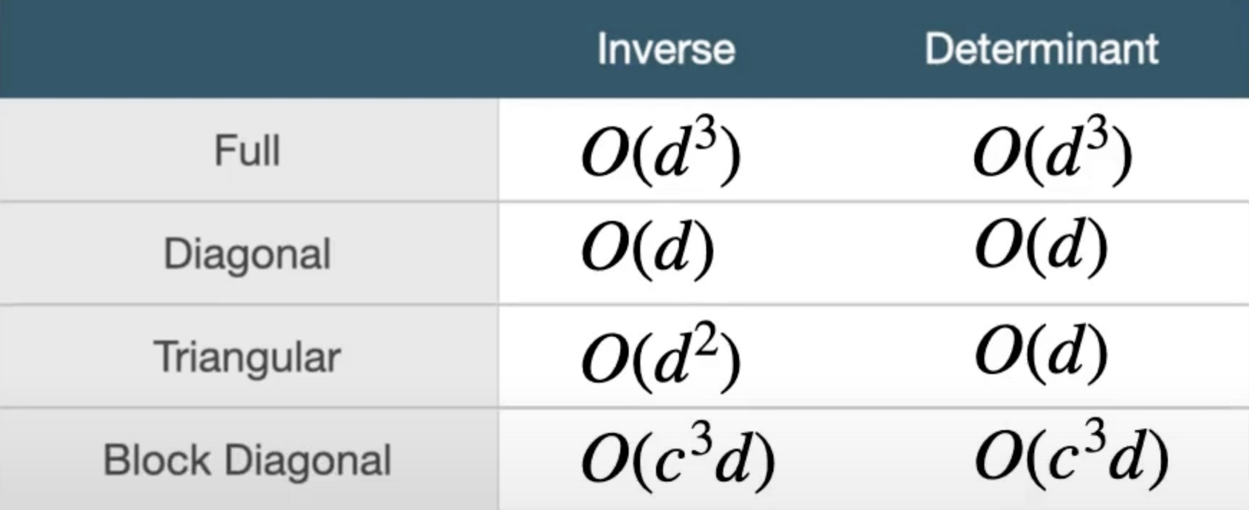
\displaystyle\left\lvert det \frac{\partial f^{-1}(x)}{\partial x}\right\rvert = det (A)
\text{Which can be computed in $O(D^3)$, as can the inverse.}
\text{Hence, using linear flows can become expensive for large D. }
Linear layer
f(z) = Az + b,
\\
\text{with $A \in \mathbb{R} ^{D \times D}$ an invertible matrix and $b \in \mathbb{R} ^{D}$}
\text{Limited in their expressiveness.}
\displaystyle\left\lvert det \frac{\partial f^{-1}(x)}{\partial x}\right\rvert = det (A)
\text{Which can be computed in $O(D^3)$, as can the inverse.}
\text{Hence, using linear flows can become expensive for large D. }
reference: https://www.youtube.com/watch?v=u3vVyFVU_lI
Coupling flows
\begin{array}{ll}
x^A &= z^A\\
x^B &= g(z^B, h(z^A)) \\
\end{array}
\\
\text{with $g(\cdot; \theta)$ a bijection}\\
\text{and $h$ any arbitrary function.}
Coupling flows
z
\begin{array}{ll}
x^A &= z^A\\
x^B &= g(z^B, h(z^A)) \\
\end{array}
\\
\text{with $g(\cdot; \theta)$ a bijection}\\
\text{and $h$ any arbitrary function.}
Coupling flows
z
z^B
z^A
\begin{array}{ll}
x^A &= z^A\\
x^B &= g(z^B, h(z^A)) \\
\end{array}
\\
\text{with $g(\cdot; \theta)$ a bijection}\\
\text{and $h$ any arbitrary function.}
Coupling flows
z
x^A
\begin{array}{ll}
x^A &= z^A\\
x^B &= g(z^B, h(z^A)) \\
\end{array}
\\
\text{with $g(\cdot; \theta)$ a bijection}\\
\text{and $h$ any arbitrary function.}
z^B
z^A
Coupling flows
z
\begin{array}{ll}
x^A &= z^A\\
x^B &= g(z^B, h(z^A)) \\
\end{array}
\\
\text{with $g(\cdot; \theta)$ a bijection}\\
\text{and $h$ any arbitrary function.}
z^B
z^A
x^A
h(z^A)
Coupling flows
z
\begin{array}{ll}
x^A &= z^A\\
x^B &= g(z^B, h(z^A)) \\
\end{array}
\\
\text{with $g(\cdot; \theta)$ a bijection}\\
\text{and $h$ any arbitrary function.}
z^B
z^A
x^A
h(z^A)
Coupling flows
z
\begin{array}{ll}
x^A &= z^A\\
x^B &= g(z^B, h(z^A)) \\
\end{array}
\\
\text{with $g(\cdot; \theta)$ a bijection}\\
\text{and $h$ any arbitrary function.}
z^B
z^A
x^A
h(z^A)
Coupling flows
z
\begin{array}{ll}
x^A &= z^A\\
x^B &= g(z^B, h(z^A)) \\
\end{array}
\\
\text{with $g(\cdot; \theta)$ a bijection}\\
\text{and $h$ any arbitrary function.}
z^B
z^A
x^A
h(z^A)
g(z^B,\: \cdot \:)
Coupling flows
z
\begin{array}{ll}
x^A &= z^A\\
x^B &= g(z^B, h(z^A)) \\
\end{array}
\\
\text{with $g(\cdot; \theta)$ a bijection}\\
\text{and $h$ any arbitrary function.}
z^B
z^A
x^A
h(z^A)
g(z^B,\: \cdot \:)
Coupling flows
z
\text{conditionner}
\begin{array}{ll}
x^A &= z^A\\
x^B &= g(z^B, h(z^A)) \\
\end{array}
\\
\text{with $g(\cdot; \theta)$ a bijection}\\
\text{and $h$ any arbitrary function.}
z^B
z^A
x^A
h(z^A)
g(z^B,\: \cdot \:)
Coupling flows
z
\text{conditionner}
\text{coupling function}
\begin{array}{ll}
x^A &= z^A\\
x^B &= g(z^B, h(z^A)) \\
\end{array}
\\
\text{with $g(\cdot; \theta)$ a bijection}\\
\text{and $h$ any arbitrary function.}
z^B
z^A
x^A
h(z^A)
g(z^B,\: \cdot \:)
Coupling flows
z
\text{conditionner}
\text{coupling function}
\text{coupling flow}
\begin{array}{ll}
x^A &= z^A\\
x^B &= g(z^B, h(z^A)) \\
\end{array}
\\
\text{with $g(\cdot; \theta)$ a bijection}\\
\text{and $h$ any arbitrary function.}
z^B
z^A
x^A
h(z^A)
g(z^B,\: \cdot \:)
Coupling flows
z
h(z^A)
g(z^B,\: \cdot \:)
\text{conditionner}
\text{coupling function}
\text{coupling flow}
\begin{array}{ll}
x^A &= z^A\\
x^B &= g(z^B, h(z^A)) \\
\end{array}
\\
\text{with $g(\cdot; \theta)$ a bijection}\\
\text{and $h$ any arbitrary function.}
z^B
z^A
x^A
Coupling flows
\text{conditionner}
\text{coupling function}
\text{coupling flow}
\text{A coupling flow is invertible if and only if $g$ is invertible.}
\begin{array}{ll}
x^A &= z^A\\
x^B &= g(z^B, h(z^A)) \\
\end{array}
\\
\text{with $g(\cdot; \theta)$ a bijection}\\
\text{and $h$ any arbitrary function.}
Coupling flows
\text{conditionner}
\text{coupling function}
\text{coupling flow}
\text{The power of a coupling flow resides in the ability of a conditioner}
\text{$h$ to be arbitrarily complex (usually modelled as a neural network).}
\begin{array}{ll}
x^A &= z^A\\
x^B &= g(z^B, h(z^A)) \\
\end{array}
\\
\text{with $g(\cdot; \theta)$ a bijection}\\
\text{and $h$ any arbitrary function.}
\text{A coupling flow is invertible if and only if $g$ is invertible.}
Coupling flows
\text{conditionner}
\text{coupling function}
\text{coupling flow}
\frac{\partial f^{-1}(x)}{\partial x} =
\begin{bmatrix}
\mathbb{I} & 0 \\
\frac{\partial g^{-1}(x^B)}{\partial x^A} & \frac{\partial g^{-1}(x^B)}{\partial x^B}
\end{bmatrix}
\begin{array}{ll}
x^A &= z^A\\
x^B &= g(z^B, h(z^A)) \\
\end{array}
\\
\text{with $g(\cdot; \theta)$ a bijection}\\
\text{and $h$ any arbitrary function.}
\text{The power of a coupling flow resides in the ability of a conditioner}
\text{$h$ to be arbitrarily complex (usually modelled as a neural network).}
\text{A coupling flow is invertible if and only if $g$ is invertible.}
Coupling flows
\text{conditionner}
\text{coupling function}
\text{coupling flow}
\begin{array}{ll}
x^A &= z^A\\
x^B &= g(z^B, h(z^A)) \\
\end{array}
\\
\text{with $g(\cdot; \theta)$ a bijection}\\
\text{and $h$ any arbitrary function.}
\implies \displaystyle\left\lvert det \frac{\partial f^{-1}(x)}{\partial x}\right\rvert = \frac{\partial g^{-1}(x^B)}{\partial x^B}
\frac{\partial f^{-1}(x)}{\partial x} =
\begin{bmatrix}
\mathbb{I} & 0 \\
\frac{\partial g^{-1}(x^B)}{\partial x^A} & \frac{\partial g^{-1}(x^B)}{\partial x^B}
\end{bmatrix}
\text{The power of a coupling flow resides in the ability of a conditioner}
\text{$h$ to be arbitrarily complex (usually modelled as a neural network).}
\text{A coupling flow is invertible if and only if $g$ is invertible.}
Coupling flows
\text{conditionner}
\text{coupling function}
\text{coupling flow}
\begin{array}{ll}
x^A &= z^A\\
x^B &= g(z^B, h(z^A)) \\
\end{array}
\\
\text{with $g(\cdot; \theta)$ a bijection}\\
\text{and $h$ any arbitrary function.}
\text{Have to choose how to split $x$.}
\implies \displaystyle\left\lvert det \frac{\partial f^{-1}(x)}{\partial x}\right\rvert = \frac{\partial g^{-1}(x^B)}{\partial x^B}
\frac{\partial f^{-1}(x)}{\partial x} =
\begin{bmatrix}
\mathbb{I} & 0 \\
\frac{\partial g^{-1}(x^B)}{\partial x^A} & \frac{\partial g^{-1}(x^B)}{\partial x^B}
\end{bmatrix}
\text{The power of a coupling flow resides in the ability of a conditioner}
\text{$h$ to be arbitrarily complex (usually modelled as a neural network).}
\text{A coupling flow is invertible if and only if $g$ is invertible.}
\text{Don't forget permutations!}
Coupling flows
Affine transformation (Real NVP)
\begin{array}{ll}
x_{1:d} &= z_{1:d}\\
x_{d+1:D} &= g(z_{d+1:D}, h(z_{1:d})) \\
&= z_{d+1:D} \odot \exp (s(z_{1:d})) + t(z_{1:d})
\end{array}
\\
\implies
\begin{array}{ll}
\displaystyle\left\lvert det \frac{\partial f^{-1}(x)}{\partial x}\right\rvert
&= \frac{\partial g^{-1}(x^B)}{\partial x^B}\\
&= \text{diag }(\exp(s(x_{1:d})))
\end{array}
\text{super easy to compute}
Other architectures
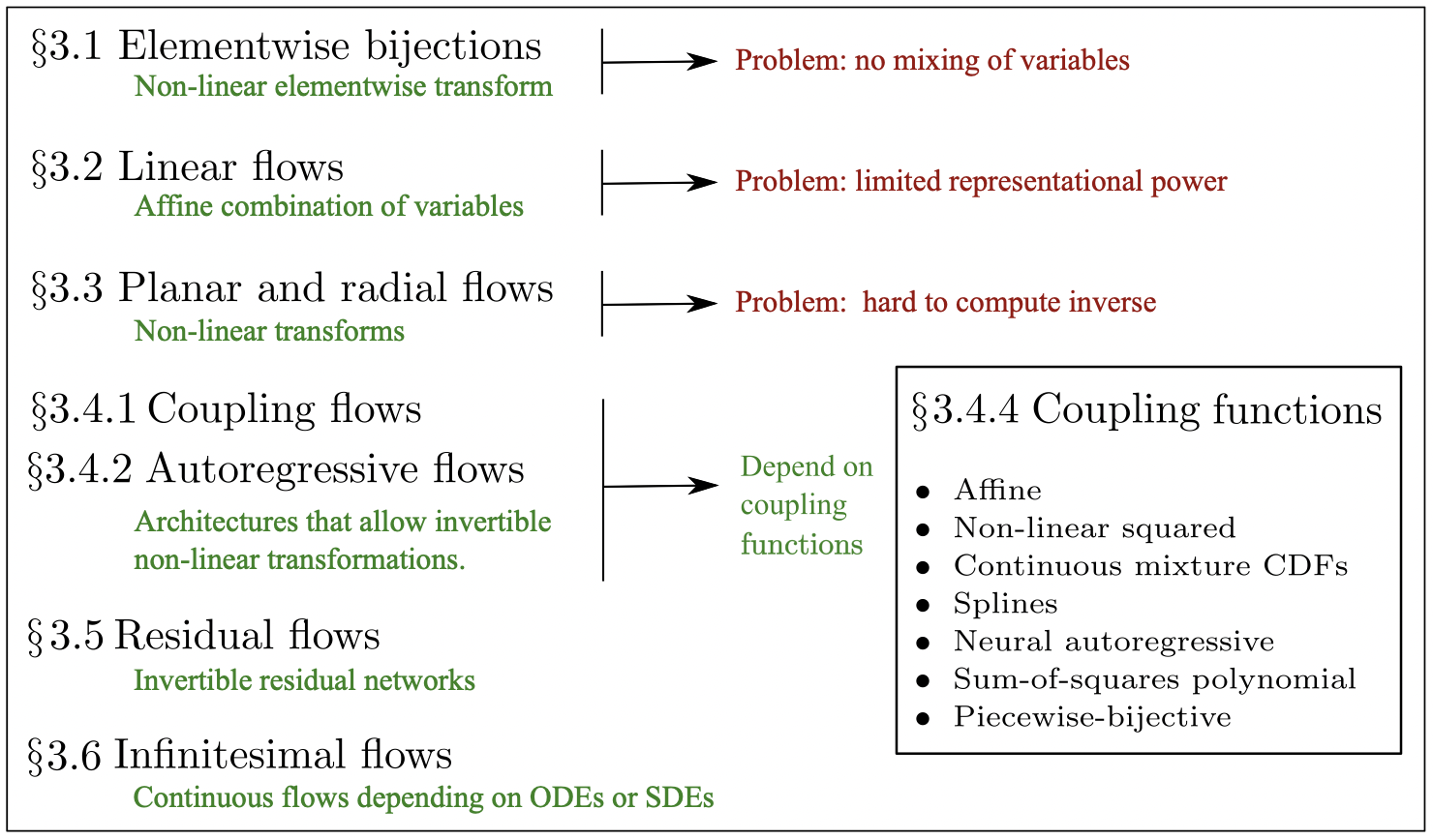
reference: https://arxiv.org/pdf/1908.09257.pdf
References
Copy of Normalizing Flows
By Andreas Tersenov


