Learning Data Science
Lecture 4
Data Science Workflow and NumPy
Functions
f
Inputs
Outputs
def c_to_f(celsius):
    return (celsius * 9/5) + 32

for temp in [0, 20, 100]:
    print(temp, "°C =", c_to_f(temp), "°F")
Typehints
- Help other users (and your future self) know the inputs and outputs
def scream(word: str, times: int) -> str:
    saying = word * times
    return saying.upper() + "!"
def scale_numbers(numbers: list[int], factor: int | float) -> list[float]:
    result = []
    for n in numbers:
        result.append(n * factor)
    return result
Docstrings
- Another way to help future you
- And especially others, if you are collaborating
def scream(word: str, times: int) -> str:
    """
    Repeat a word several times and return it in uppercase with an exclamation mark.

    Parameters
    ----------
    word : str
        The word to repeat.
    times : int
        How many times to repeat the word.

    Returns
    -------
    str
        The repeated word in uppercase, followed by an exclamation mark.

    Examples
    --------
    >>> scream("ha", 3)
    'HAHAHA!'
    """

    saying = word * times
    return saying.upper() + "!"
There are many ways to format docstrings
This one is called the numpy style
Exceptions
- Python's way of telling us something is wrong
- They stop your program!

def circle_area(radius: float) -> float:

    if radius < 0:
        raise ValueError("Radius cannot be negative.")

    return 3.1415 * radius ** 2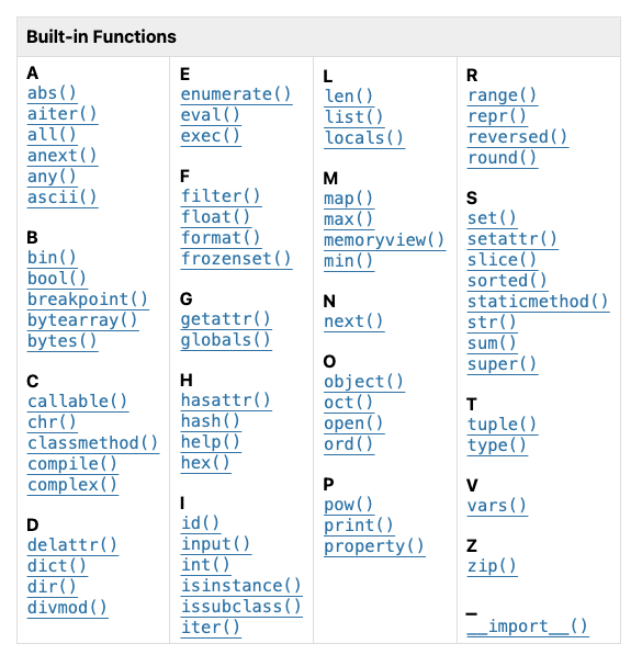
import time

time.sleep(5)

# or you can import just one function
from time import sleep

sleep(5)

# nickname a module/function
import time as t

t.sleep(5)
Python Builtin Functions and Modules
class Character:
    """A character in our video game."""

    def __init__(self, name: str, base_health: int):
        # ...
        self.name = name
        self.base_health = base_health
        self.items: list[str] = []

    def pickup_item(self, item: str):
        """
        Add an item to the character's inventory.

        Parameters
        ----------
            item : str
                The item to pick up
        """
        self.items.append(item)
Character
-
name
-
health
-
items
-
pickup_item()
warrior = Character(name="Hodor", health=100)

print(warrior.items)

warrior.pickup_item("sword")

print(warrior.items)
Objects
"nouns"
"verbs"
Debugging
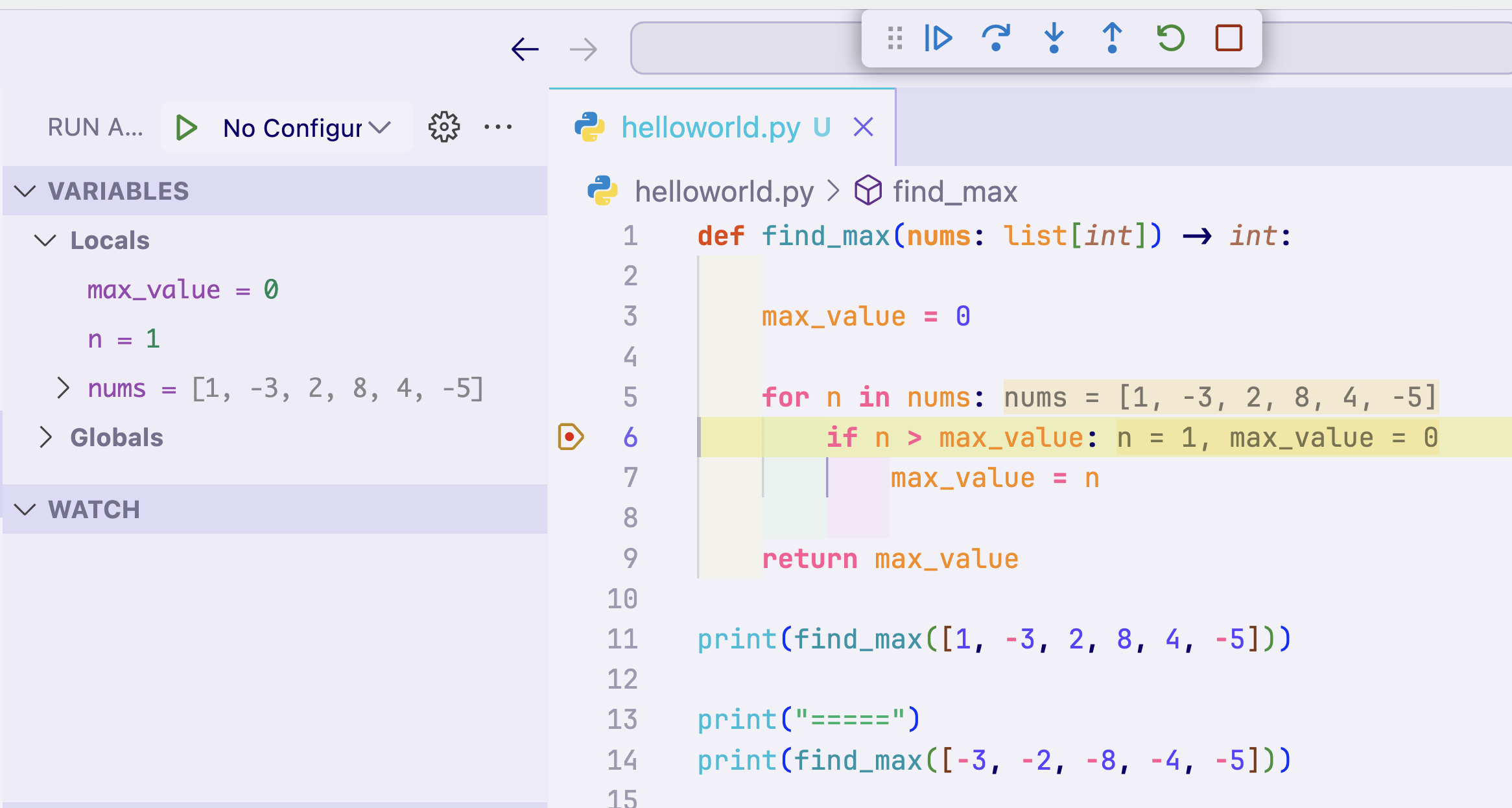
- Debugging helps you efficiently find where errors or strange behaviors arise in your code
Debugging in VS Code
Lecture 4
- Recap
- Project Scaffolding with uv
- Python Notebooks
- Linear Algebra in a Nutshell
- NumPy Fundamentals
Project Scaffolding
- Where do you start when beginning a new project?
- How do you install external packages?
- All can be easily done with uv
Let's work through it together!
Project Scaffolding
1. Create a new folder 'ds-lecture-4' in your projects directory. This will be the root of today's work.
2. Open this folder with VS Code
3. Run the command:
uv init -p 3.13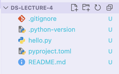
By the end you should see these files

4. Run the command:
- this will create the virtual environment
5. If the following popup appears, always say yes!
- if it doesn't appear, use the command palette
Project Scaffolding
uv sync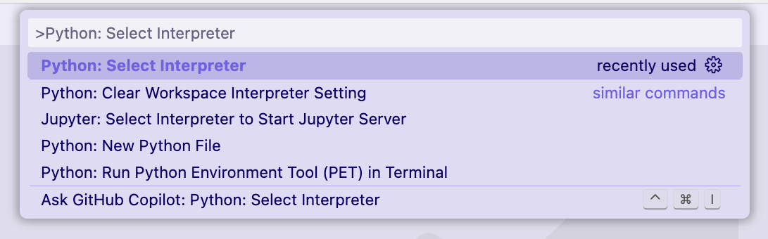
Everything here is review from Lecture 2 :)
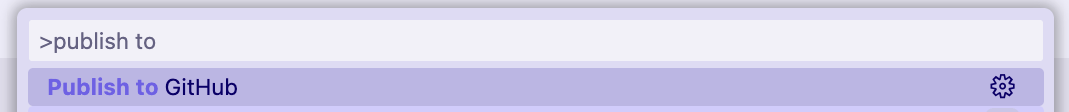
6. Use the command palette to select "Publish to GitHub"
- you can choose if you want your code to be public or private
Adding a new project to your GitHub
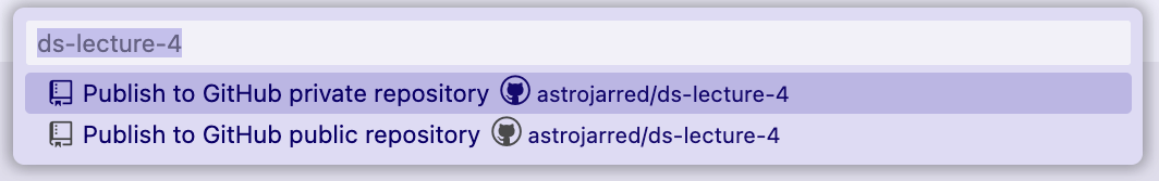
Your repository is available now at github.com/username/ds-lecture-4 ✨
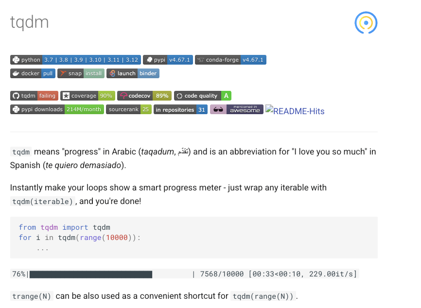
7. Let's install the 'tqdm' package to our environment
- It allows you to create loading bars
- Not built into Python, so we have to add it!
Adding external packages
uv add tqdm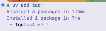
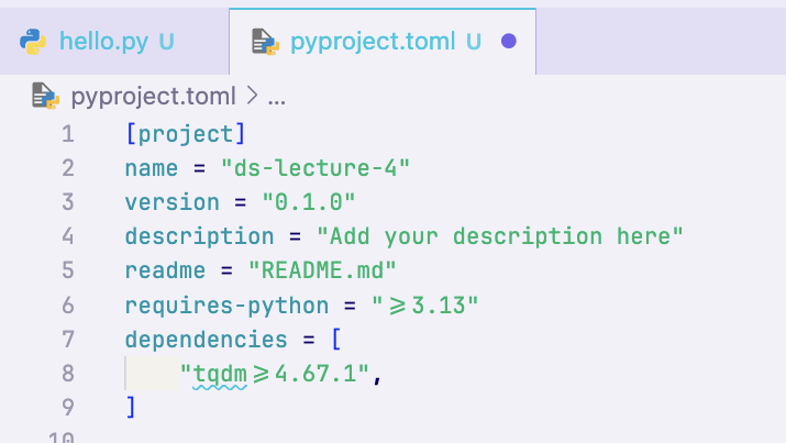
tqdm got added to pyproject.toml !
8. Try using tqdm in a small script to test that it worked
Adding external packages
from tqdm import tqdm

for i in tqdm(range(30000000)):
    pass

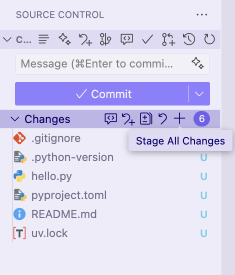
9. Sync our changes to GitHub
- Now we can use the VS Code UI to save time ✨
Adding external packages
- Open the Version Control tab
- Click the + button to add all files
- Note: you could also select individual files or even individual lines of code
- Type a commit message (e.g. "First commit") and click Commit
- Push the changes to GitHub:

And that's how you start a project and install packages with uv!
Lecture 4
- Recap
- Project Scaffolding with uv
- Python Notebooks
- Linear Algebra in a Nutshell
- NumPy Fundamentals
Python Notebooks
Ways to interact with Python code
REPL
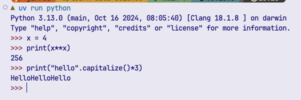
✅ Interactive
❌ Sharable
❌ Version Control friendly
❌ Reproducible
❌ Mix code, text, plots
Scripts
❌ Interactive
✅ Sharable
✅ Version Control friendly
✅ Reproducible
❌ Mix code, text, plots
Notebooks
✅ Interactive
✅ Sharable
⚠️ Version Control friendly
⚠️ Reproducible
✅ Mix code, text, plots
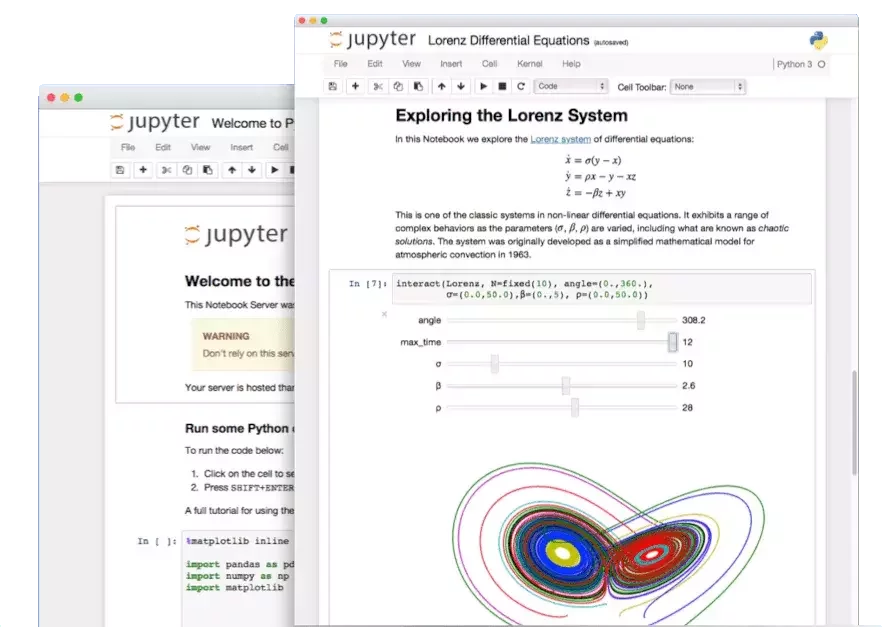
Python Notebooks
Python Notebooks
- Interactive files where you can
- Run Python code
- Create images and plots
- Take notes with Markdown
- All inside one file!
⚠️ Reproducing results
⚠️ Tracking changes with Git
⚠️ Scalability
⚠️ Performance
✅ Playing with data
✅ Taking nodes
✅ Making plots
✅ Interactive
✅ Good for demos
Notebooks in VS Code
Do it!
- Open VS Code to a new project folder
- Add the package ipykernel to your project with uv
- Find and install the Jupyter extension
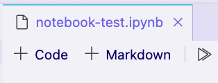
- Create a new file called "test.ipynb"
- Create a Markdown cell and make a header
- Create a code cell and add a Hello World

3.
6.
5.
ipynb = Interactive Python Notebook
Notebooks in VS Code
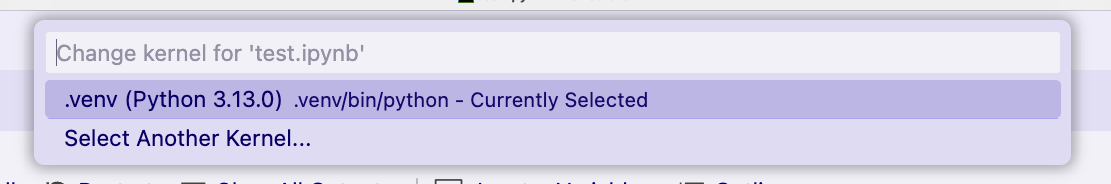
When you first try to run a cell with code, it will ask you to select your interpreter again.
Remember to use the one located at
.venv
Notebooks in VS Code
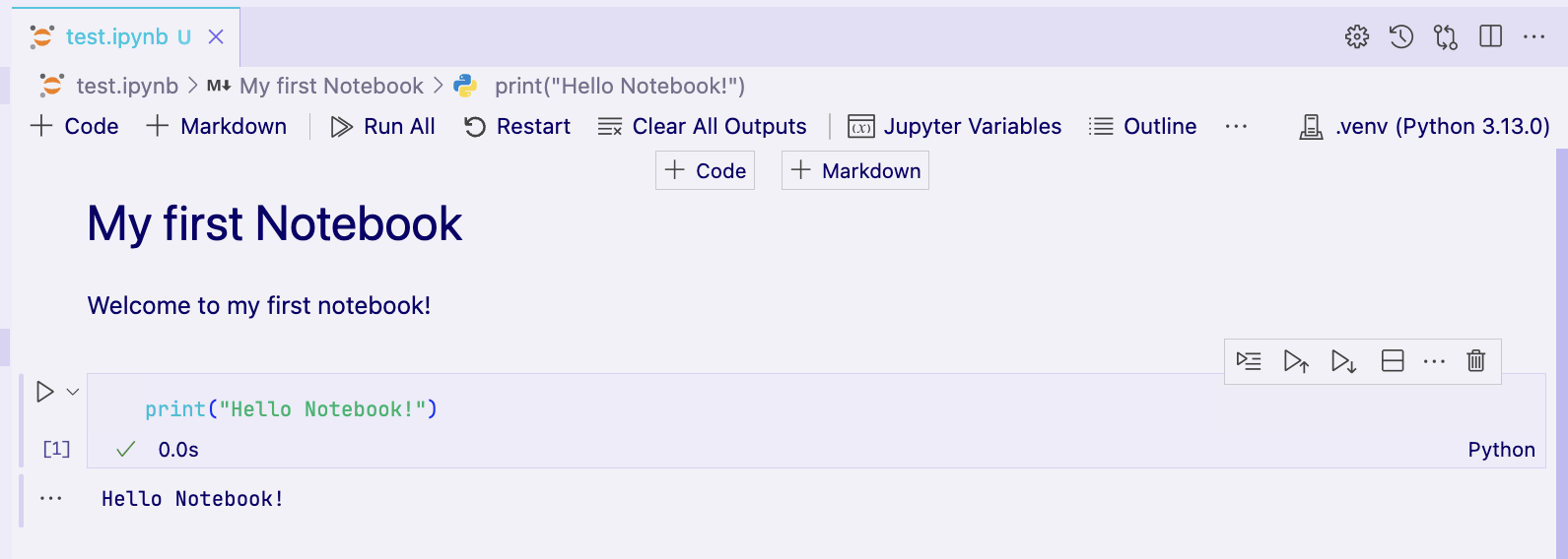
Add a code cell
Add a markdown cell
Run all notebook cells sequentially
Run this cell only
Delete this cell
Switch this cell between python/markdown
Restart the notebook (all imports and variables lost)
Lecture 4
- Recap
- Project Scaffolding with uv
- Python Notebooks
- Linear Algebra in a Nutshell
- NumPy Fundamentals
Linear Algebra
The math of vectors and matrices
How to combine and transform them
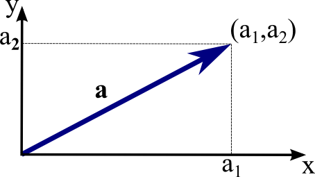
What is a vector?
A vector is a list of numbers.
That's it ✨
Many concepts and physical quantities can be expressed in terms of vectors
What is a vector?
A vector is a list of numbers.
That's it ✨
Coordinates
Data
Equations

4x^2 + 2x + 1 = 0
[4, 2, 1]
[x, y]
[4, 7, 8, 2]
What is a vector?
Vectors don't live in isolation:
there is usually some underlying information
Coordinates
Data
Equations
[x, y]
[4, 7, 8, 2]
4x^2 + 2x + 1 = 0
[4, 2, 1]
Spatial coordinates and origin is assumed [0, 0]
Units are luminosity and data is captured every 1s
Numbers represent coefficients of a polynomial
Vector Math at a Glance
addition / subtration
\mathbf{a} \pm \mathbf{b} = [a_1 \pm b_1,\ a_2 \pm b_2,\ ...]
vector multiplication
c\mathbf{a} = [ca_1,\ ca_2,\ ...]
\mathbf{a} \odot \mathbf{b} = [a_1 b_1,\ a_2 b_2,\ ...]
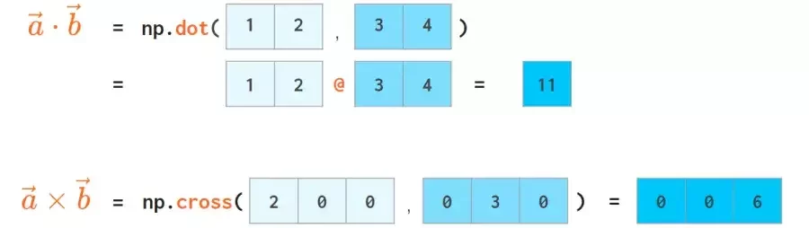
dot product
\mathbf{a} \cdot \mathbf{b} = \sum_i a_i b_i = a_1 b_1\ + a_2 b_2\ + ...
magnitude / norm
··||\mathbf{a}|| = \sqrt{\mathbf{a} \cdot \mathbf{a}} = \sqrt{\sum_i a_i^2}
√
Challenge #1
Challenge #1
\mathbf a=[1,\,2], \mathbf b=[3,\,-1]
Pen and paper exercises
find:
\mathbf a \cdot \mathbf b = \, ?
|| \mathbf b || = \, ?
What is a Matrix?
Multiple vectors stacked together?
This can represent higher-order information
Coordinates ➡️ many points at once
What is a Matrix?
\begin{bmatrix}
x_1 & x_2 & x_3 & ... & x_n \\
y_1 & y_2 & y_3 & ... & y_n \\
\end{bmatrix}
pair of coordinates
Matrix as a transformation
What is a Matrix?
\begin{bmatrix}
2 & 0 \\
0 & 3 \\
\end{bmatrix}
=
\begin{bmatrix}
2x \\
3y \\
\end{bmatrix}
\begin{bmatrix}
x \\
y \\
\end{bmatrix}
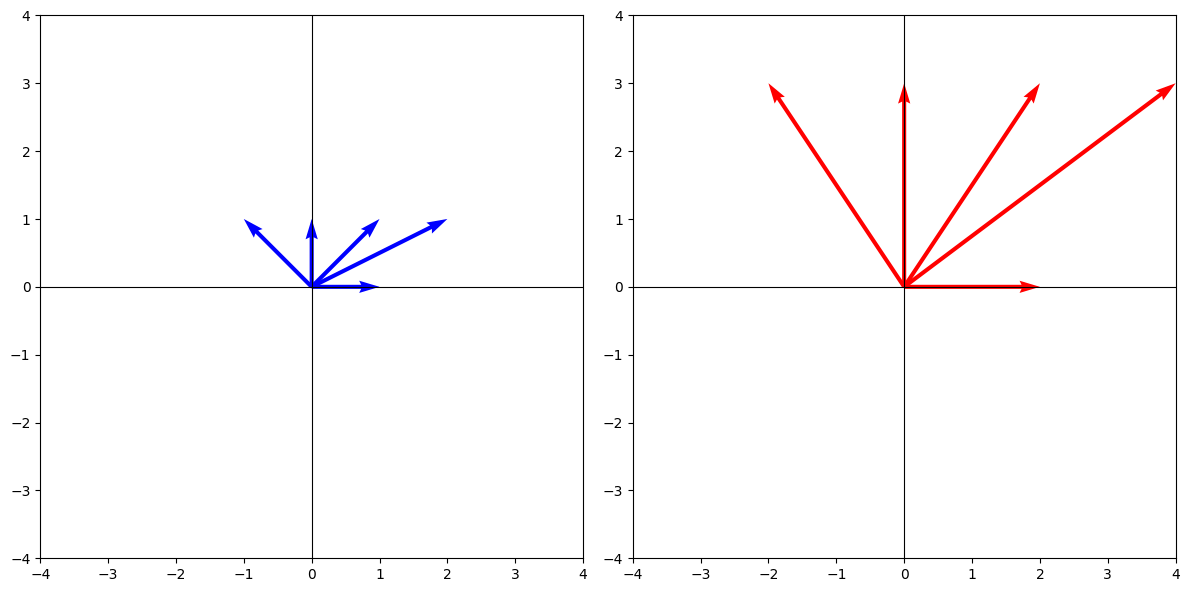
\begin{bmatrix}
2 & 0 \\
0 & 3 \\
\end{bmatrix}
Matrix as data with attributes
What is a Matrix?
Data=\begin{bmatrix}
\text{lum}_1 & \text{freq}_1 & \text{snr}_1\\
\text{lum}_2 & \text{freq}_2 & \text{snr}_2\\
\text{lum}_3 & \text{freq}_3 & \text{snr}_3\\
\text{lum}_4 & \text{freq}_4 & \text{snr}_4
\end{bmatrix}
Each row in the matrix is a one data point
Parameters of multiple functions
What is a Matrix?
\begin{aligned}
y_1 &= 2x_1 + 3x_2 + 1 \\
y_2 &= -x_1 + 4x_2 - 2 \\
y_3 &= 0.5x_1 - x_2 + 0
\end{aligned}
Parameters of multiple functions
What is a Matrix?
\begin{aligned}
y_1 &= 2x_1 + 3x_2 + 1 \\
y_2 &= -x_1 + 4x_2 - 2 \\
y_3 &= 0.5x_1 - x_2 + 0
\end{aligned}
\mathbf{y} =
\mathbf{A}
\mathbf{x}
+
\mathbf{b}
\mathbf{y} =
\begin{bmatrix}
2 & 3 \\
-1 & 4 \\
0.5 & -1
\end{bmatrix}
\begin{bmatrix}
x_1 \\
x_2
\end{bmatrix}
+
\begin{bmatrix}
1 \\
-2 \\
0
\end{bmatrix}
\mathbf{A}
\mathbf{x}
\mathbf{b}
+
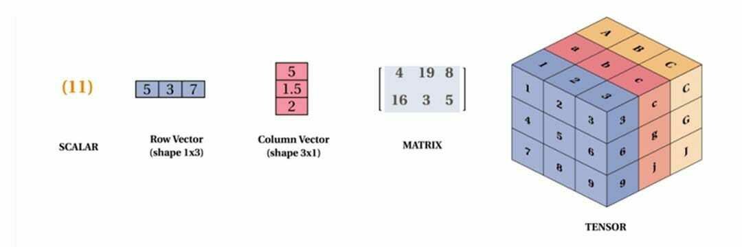
What is a Tensor?
Multiple matrices stacked together.
A higher-order matrix.
What is a Tensor?
Rank 0
Tensor
Rank 1
Tensors
Rank 2
Tensor
Rank 3
Tensors
Everything is a tensor

Color images are tensors!
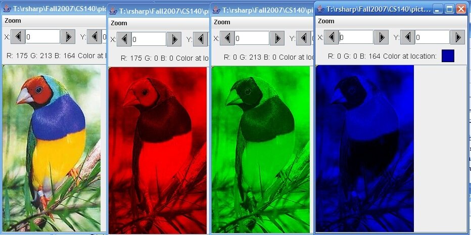
Graphics from: St. Lawrence U CS140 and Montesinos-López et al (2022)
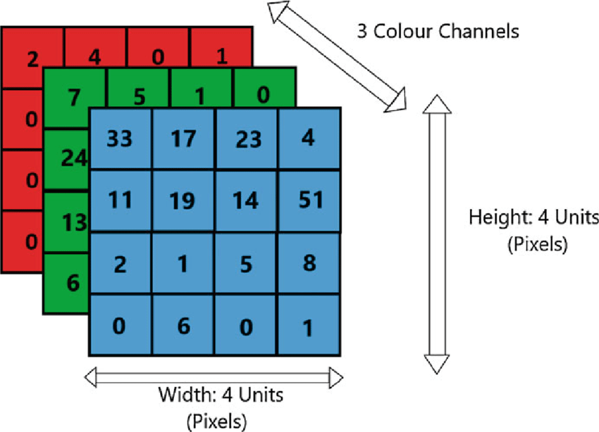
Image width (4px)
Image height (4px)
Image "depth"
(3 color channels)
Metrix Math at a Glance
matrix x vector
\mathbf{A} \mathbf{x} = \mathbf{Y}
matrix multiplication
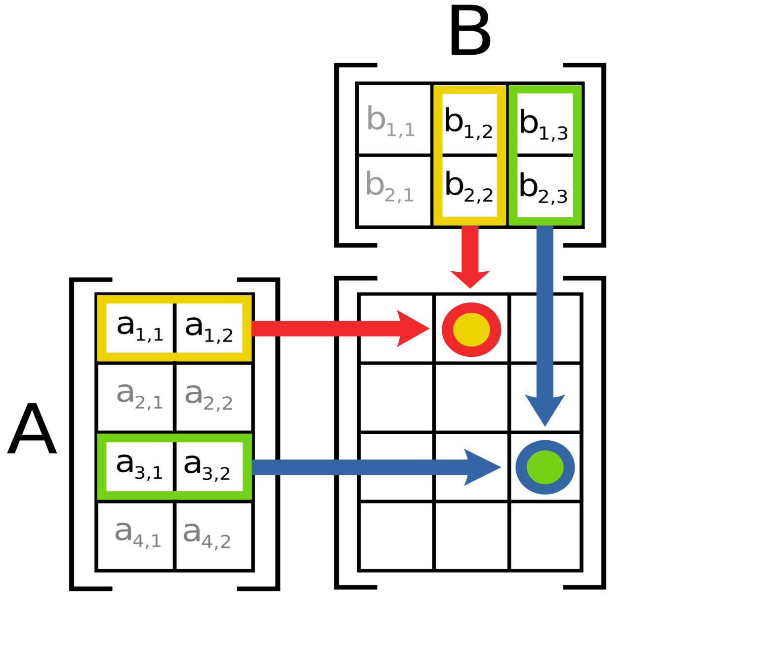
\text{cell}\ c_{ij} = \sum_{k=1}^n a_{ik} b_{kj}
C
\mathbf{AB} = \mathbf{C}
Metrix Math at a Glance
transpose
\mathbf{A} \rightarrow \mathbf{A^T}
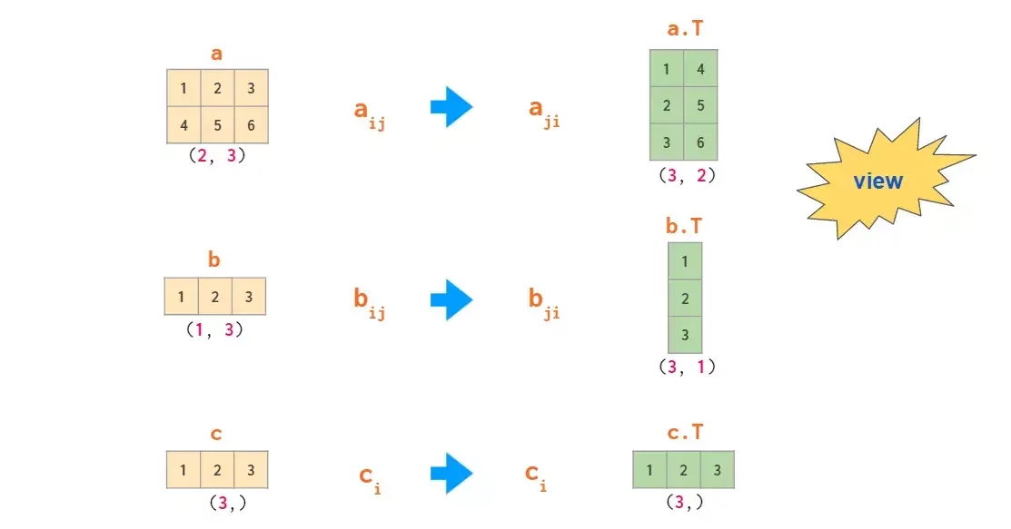
*flips matrix along main diagonal*
\mathbf{A} = \mathbf{(A^T)^T}
it's inversable
Now let's put it all together:
jupyter + linear algebra
✨
Lecture 4
- Recap
- Project Scaffolding with uv
- Python Notebooks
- Linear Algebra in a Nutshell
- NumPy Fundamentals
NumPy
💻 The rest of today's lecture will be spent learning NumPy.
Open up a new notebook which you can use for note-taking and completing challenges
Please install NumPy with
uv add numpy
What is NumPy?
NumPy is array library that powers all of scientific Python
Fancy lists
NumPy Superpowers:
⚡️ Vectorization
⚡️ Broadcasting
⚡️ Fassssst
We'll come to these later
Lists need loops
my_list = [1,2,3,4,5]

print(my_list ** 2)
# raises an Error!
import numpy as np
my_array = np.array([1,2,3,4,5])
print(my_array**2)my_list = [1,2,3,4,5]
squared = []
for i in my_list:
squared.append(i**2)
# OR
squared = [i**2 for i in my_list]
print(squared)Solution using lists
Solution using numpy
Vectorization
import numpy as np

my_array = np.array([1,2,3,4,5])

print(my_array**2)
# array([ 1, 4, 9, 16, 25])This is called vectorization ✨
Operations on vectorized objects are:
- faster
- no loops involved
- easier for the user
print(my_array + 5)
# array([ 6,  7,  8,  9, 10])
other = np.array([6,7,8,9,10])
print(my_array + other)
# array([ 7, 9, 11, 13, 15])What is NumPy?
NumPy is array library that powers all of scientific Python
Fancy lists
Fancy linear algebra
You can put arrays in arrays to create/manipulate vectors, matrices, and tensors
You can put arrays in arrays to create/manipulate vectors, matrices, and tensors
Later we'll see how it makes sense to manipulate data as vectors and matrices
This will be super important for the ML section next week as well!
Challenge #1
Challenge #1
import numpy as np

my_array = np.array([1, 2, 3, 4, 5])
other = np.array([6, 7, 8, 9, 10])- Find a way to do element-wise multiplication of the two lists without numpy
- Then try again using numpy arrays
- Which is easier?
my_list    = [1, 2, 3, 4, 5]
other_list = [6, 7, 8, 9, 10]
With normal lists
With numpy arrays
# expected result
[ 6 14 24 36 50 ]
Next up: 1D arrays (aka Vectors)
Array Attributes
Easily get the type or shape of an array
my_array = np.array([1,2,3,4,5])
print(my_array.dtype)   # int64
print(my_array.shape)   # (5)

my_array = np.array([1,2,3,4,5], dtype=float)
print(my_array.dtype)   # float64
Array Creation Patterns
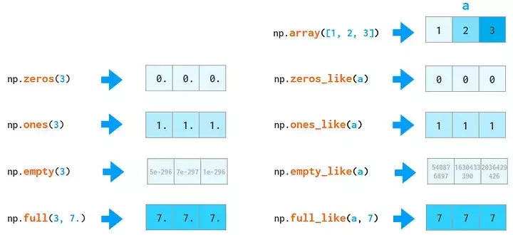
print(np.ones(6))

# [1 1 1 1 1 1]
Array Creation Patterns
You can also create arrays that are the same size as an already-existing one
my_array = np.array([1,2,3,4,5])
print(np.ones_like(my_array))

# [1 1 1 1 1]
Initializing With Sequences
Random Arrays
my_array = [6, 89, 384]

rng = np.random.default_rng()
rng.choice(my_array)
# 89

# can pass probabilities
rng.choice(my_array, p=[0.1, 0.1, 0.8])
# 384 (probably ;)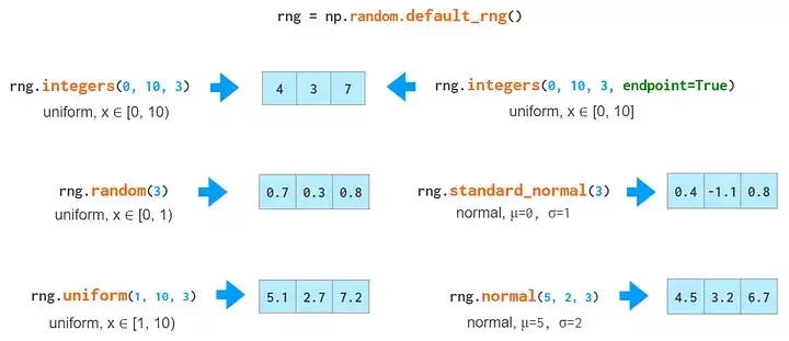
Challenge #2
Challenge #2
Create a function that uses numpy to generate n random numbers
between -1 and +1
# expected result
print(my_rand(n=3))
# [-0.348, 0.894, -0.028]
Reproducible Randomness
- Sometimes (ie testing purposes), you want the same answer from an RNG
- You can pass a seed
rng = np.random.default_rng()
print(f"Seed: {rng.bit_generator.seed_seq.entropy}")
print(rng.random(5))

Seed: 121739455997546233386808762441738277564
[0.7538113  0.33547651 0.08440574 0.97809579 0.06358138]

rng2 = np.random.default_rng()
print(f"Seed: {rng2.bit_generator.seed_seq.entropy}")
print(rng2.random(5))

Seed: 187878457149970364692539552433862812938
[0.24586211 0.91028715 0.23901012 0.56294228 0.25043037]
No seed provided
Reproducible Randomness
- Sometimes (ie testing purposes), you want the same answer from an RNG
- You can pass a seed
rng = np.random.default_rng(42)  # <--- seed is 42
print(f"Seed: {rng.bit_generator.seed_seq.entropy}")
print(rng.random(5))

Seed: 42
[0.77395605 0.43887844 0.85859792 0.69736803 0.09417735]

rng2 = np.random.default_rng(42)
print(f"Seed: {rng2.bit_generator.seed_seq.entropy}")
print(rng2.random(5))

Seed: 42
[0.77395605 0.43887844 0.85859792 0.69736803 0.09417735]
Seed provided: 42
Vector Indexing
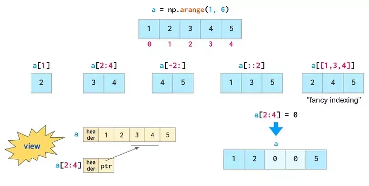
Not too different from lists
Main difference: editing a slice of an array, changes the original!
a = np.arange(1, 6)
# [1 2 3 4 5]

a[2:4] = 0
print(a)
# [1 2 0 0 5]
Boolean Indexing
Logical operations on arrays
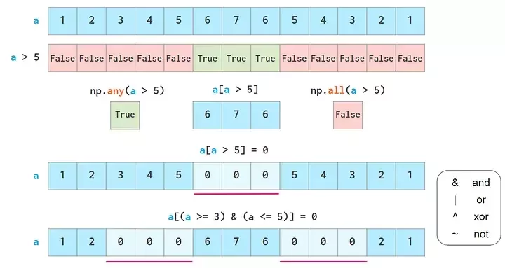
# boolean indexing
a = np.array([1, 2, 3, 4, 5, 4, 3, 2, 1])
print(a > 3)
# [False False False True True False False False False]
a[a > 3] = 0
print(a)
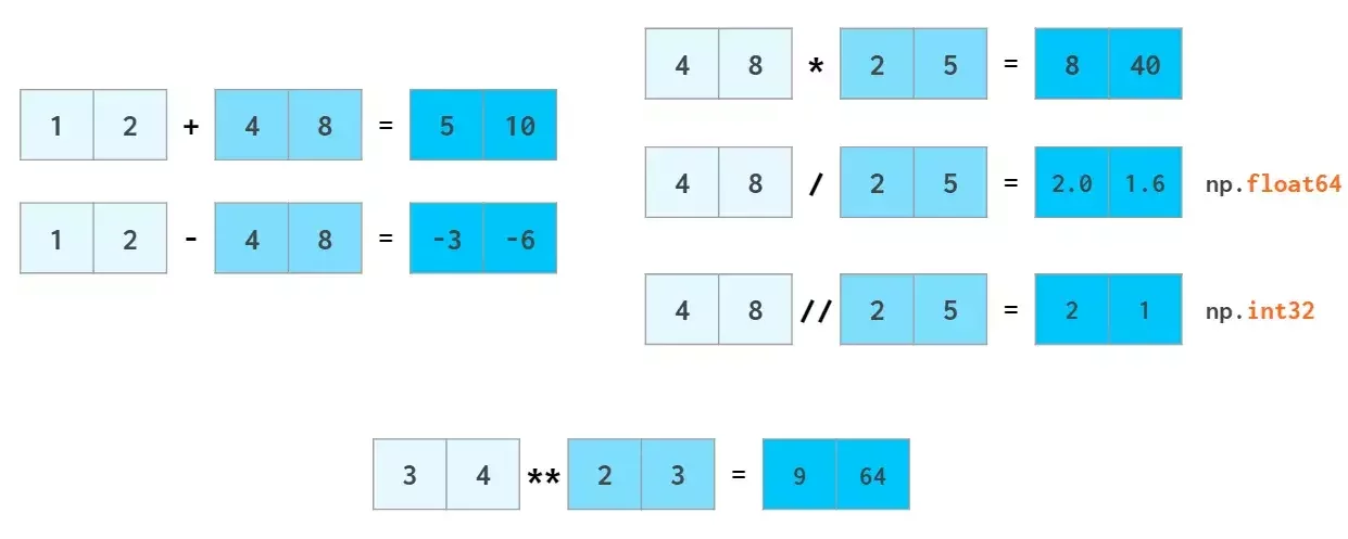
# [1 2 3 0 0 0 3 2 1]Vector Math
- We already touched on this a bit
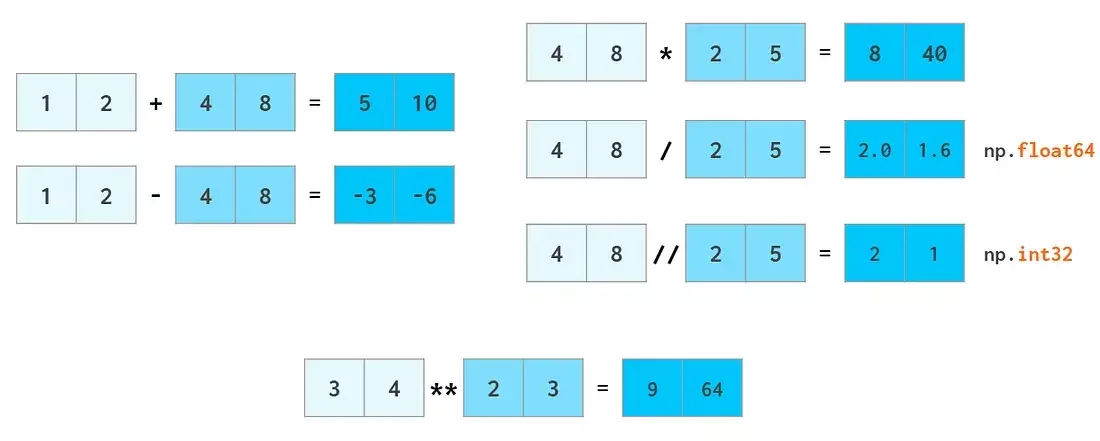
Element-wise operations between two arrays
Vector Math
- We already touched on this a bit
Element-wise operations between one array and one number (scalar)
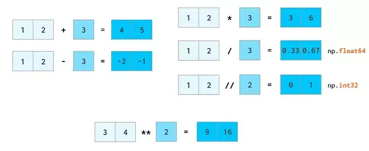
This is called broadcasting ✨
In these cases, the scalar gets 'promoted' to an array behind the scenes
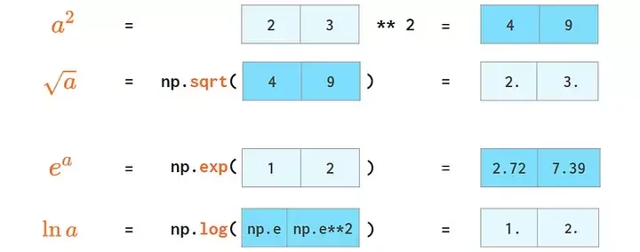
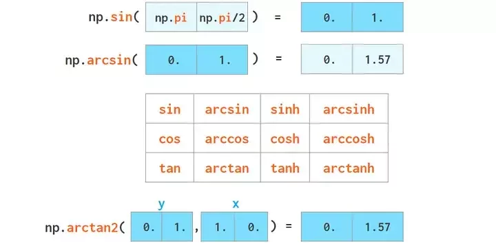
Vector Math
Most functions from the built-in `math` module also are in numpy and work on arrays!
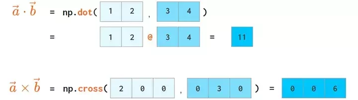
Vector Math
Linear algebra 😱
Vector Math
Stats! 😱
Challenge #3
Challenge #3
- Using numpy arrays, calculate the sin^2 of every integer degree in [0, 360] deg
- Then find the mean and standard deviation of this array
- No for loops allowed!
Vectors / 1D arrays review
x = np.array([1,2,3,4,5])
# OR
l = [1, 2, 3, 4, 5]
x = np.array(l)
Create an array
x = np.ones(5)
x = np.zeros(5)
Initialize an array
x = np.array([1,2,3,4,5])
y = np.ones_like(x)
Initialize from another array's shape
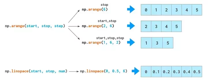
x = np.arange(6)
x = np.arange(1, 6, 2)
x = np.linspace(0, 1, 11)
Initialize a sequence
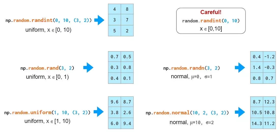
rng = np.random.default_rng()
# 5 ints between [0,100)
rng.integers(0, 100, 5)

# 10 ints between [0, 1)
rng.random(10)

# 6 samples from a gaussian
# mean=5, std=3
rng.normal(5, 3, 6)
Random number generator
x = np.arange(1, 6)
# [1, 2, 3, 4, 5]
x[1] # = 2
x[2:4] # = [3, 4]
# everything from index -2 and onwards
x[-2:] # = [4, 5]
# Every 2 indices (step=2)
x[::2] # = [1, 3, 5]
# specifically indicies 1, 3, 4
x[[1, 3, 4]] # = [2, 4, 5]
Indexing
x = np.array([1, 2])
y = np.array([3, 6])
x + y # = [4, 8]
x * y # = [3, 12]
x + 2 # = [3, 4]
np.sqrt(x)
np.sin(x)
Vector operations
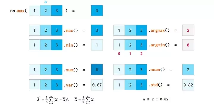
x.max()
x.sum()
x.mean()
# etc
Stats
Matrices, 2D Arrays
Matrices
In NumPy, matrices are arrays inside an array!
np.array([1, 2, 3])
x.shape  # (3)
1D Array / Vector
np.array([1, 2, 3])
x.shape  # (3)
np.array([1, 2, 3])
x.shape # (3)2D Array / Matrix
x = np.array([
    [1, 2, 3],
    [4, 5, 6]
])
x.shape  # (2, 3)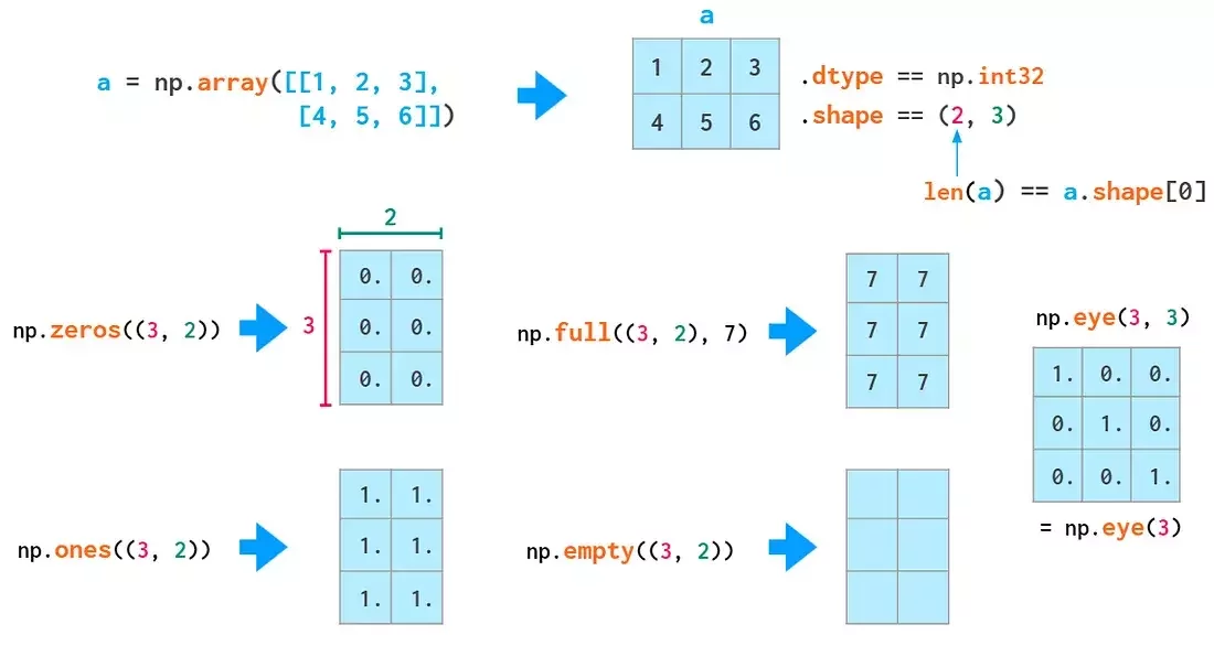
("rows", "columns")
Matrix Initialization
Most logic from 1D cases can be expanded
Indexing syntax
[row, column]
: means 'all'
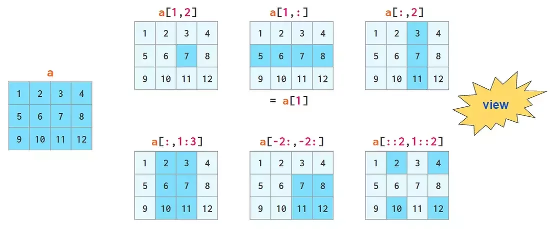
(3, 4)
First row,
every element
Every row,
second element
First row,
second col
Let's pretend this matrix represents student grades
Susie
Jay
Lara
| Trig. | Alg. | Geom. | Calc. |
|---|---|---|---|
| 1.3 | 1.3 | 3.7 | 2.3 |
| 4.0 | 4.3 | 2.0 | 2.3 |
| 1.3 | 1.0 | 2.0 | 3.0 |
Indexing syntax
[row, column]
: means 'all'
Jay's Geometry Grade
Susie
Jay
Lara
| Trig. | Alg. | Geom. | Calc. |
|---|---|---|---|
| 1.3 | 1.3 | 3.7 | 2.3 |
| 4.0 | 4.3 | 2.0 | 2.3 |
| 1.3 | 1.0 | 2.0 | 3.0 |
(3, 4)
First row,
every element
Every row,
second element
First row,
second col
Indexing syntax
[row, column]
: means 'all'
All Jay's Grades
Susie
Jay
Lara
| Trig. | Alg. | Geom. | Calc. |
|---|---|---|---|
| 1.3 | 1.3 | 3.7 | 2.3 |
| 4.0 | 4.3 | 2.0 | 2.3 |
| 1.3 | 1.0 | 2.0 | 3.0 |
(3, 4)
First row,
every element
Every row,
second element
First row,
second col
Indexing syntax
[row, column]
: means 'all'
All Geometry Grades
Susie
Jay
Lara
| Trig. | Alg. | Geom. | Calc. |
|---|---|---|---|
| 1.3 | 1.3 | 3.7 | 2.3 |
| 4.0 | 4.3 | 2.0 | 2.3 |
| 1.3 | 1.0 | 2.0 | 3.0 |
(3, 4)
First row,
every element
Every row,
second element
First row,
second col
The Axis Argument
a.sum() =
Susie
Jay
Lara
| Trig. | Alg. | Geom. | Calc. |
|---|---|---|---|
| 1.3 | 1.3 | 3.7 | 2.3 |
| 4.0 | 4.3 | 2.0 | 2.3 |
| 1.3 | 1.0 | 2.0 | 3.0 |
= 28.5
Susie
Jay
Lara
| Trig. | Alg. | Geom. | Calc. |
|---|---|---|---|
| 1.3 | 1.3 | 3.7 | 2.3 |
| 4.0 | 4.3 | 2.0 | 2.3 |
| 1.3 | 1.0 | 2.0 | 3.0 |
a =
grades = np.array([
    [1.3, 1.3, 3.7, 2.3],
    [4.0, 4.3, 2.0, 2.3],
    [1.3, 1.0, 2.0, 3.0]
])
a.sum(axis=0) =
Susie
Jay
Lara
= [6.6, 6.6, 7.7, 7.6]| Trig. | Alg. | Geom. | Calc. |
|---|---|---|---|
| 1.3 | 1.3 | 3.7 | 2.3 |
| 4.0 | 4.3 | 2.0 | 2.3 |
| 1.3 | 1.0 | 2.0 | 3.0 |
a.sum(axis=1) =
Susie
Jay
Lara
= [8.6, 12.6, 7.3]| Trig. | Alg. | Geom. | Calc. |
|---|---|---|---|
| 1.3 | 1.3 | 3.7 | 2.3 |
| 4.0 | 4.3 | 2.0 | 2.3 |
| 1.3 | 1.0 | 2.0 | 3.0 |
The Axis Argument
Susie
Jay
Lara
| Trig. | Alg. | Geom. | Calc. |
|---|---|---|---|
| 1.3 | 1.3 | 3.7 | 2.3 |
| 4.0 | 4.3 | 2.0 | 2.3 |
| 1.3 | 1.0 | 2.0 | 3.0 |
a =
grades = np.array([
    [1.3, 1.3, 3.7, 2.3],
    [4.0, 4.3, 2.0, 2.3],
    [1.3, 1.0, 2.0, 3.0]
])
Tabular data (i.e. row/column data) is naturally represented as a 2D matrix!
- Row: each data sample
- Column: each feature (i.e. attribute) in your data
Challenge #4
Challenge #4
Copy the data from the code block below
- What is the shape of the data (amounts matrix), and what does each axis represent?
- How many fruits were sold in total over this week?
- Which day sold the most fruits?
- Which fruit was the best seller?
fruits = np.array([
    "apples",
    "bananas",
    "cherries",
    "dates",
    "elderberries",
    "figs",
    "grapes",
    "huckleberries",
    "kiwis",
    "lemons",
    "mangos",
    "nectarines",
])

# amount sold per weekday
amounts = np.array([
    [10, 20, 30, 40, 50, 60, 70],
    [15, 25, 35, 45, 55, 65, 75],
    [20, 30, 40, 50, 60, 70, 80],
    [25, 35, 45, 55, 65, 75, 85],
    [30, 40, 50, 60, 70, 80, 90],
    [10, 24, 30, 36, 42, 48, 54],
    [10, 20, 30, 40, 50, 60, 70],
    [4, 8, 12, 16, 20, 24, 28],
    [1, 2, 3, 4, 5, 6, 7],
    [3, 5, 7, 9, 11, 13, 15],
    [1, 4, 7, 10, 13, 16, 19],
    [34, 12, 23, 12, 23, 12, 23],
])
Note: The week starts from Monday-Sunday
Matrix Math
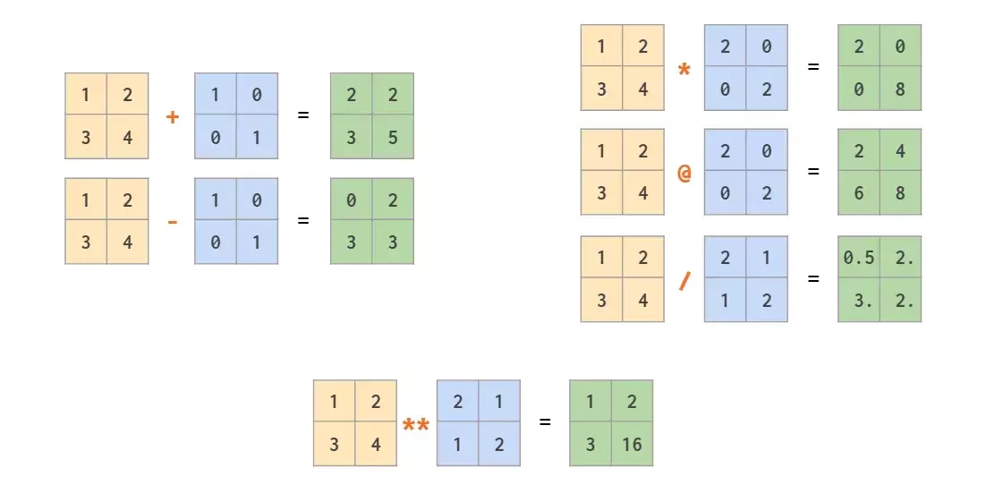
All element-wise except :
- @ is a special operator for matrix product
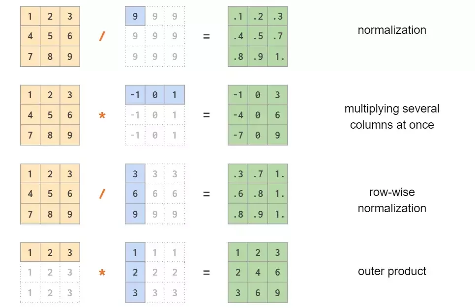
More Matrix Math

Normalization
Multiplying several columns
Row-wise normalization
Outer Product
This all must seem very overwhelming, like a lot to remember!
But you don't have to memorize any of this.
You will get used to this notation as you use it, and can look things up as you go along 💫
Creating Matrices from Arrays
When you have a single, long array and you want to turn it into a matrix:
Use the reshape() method!
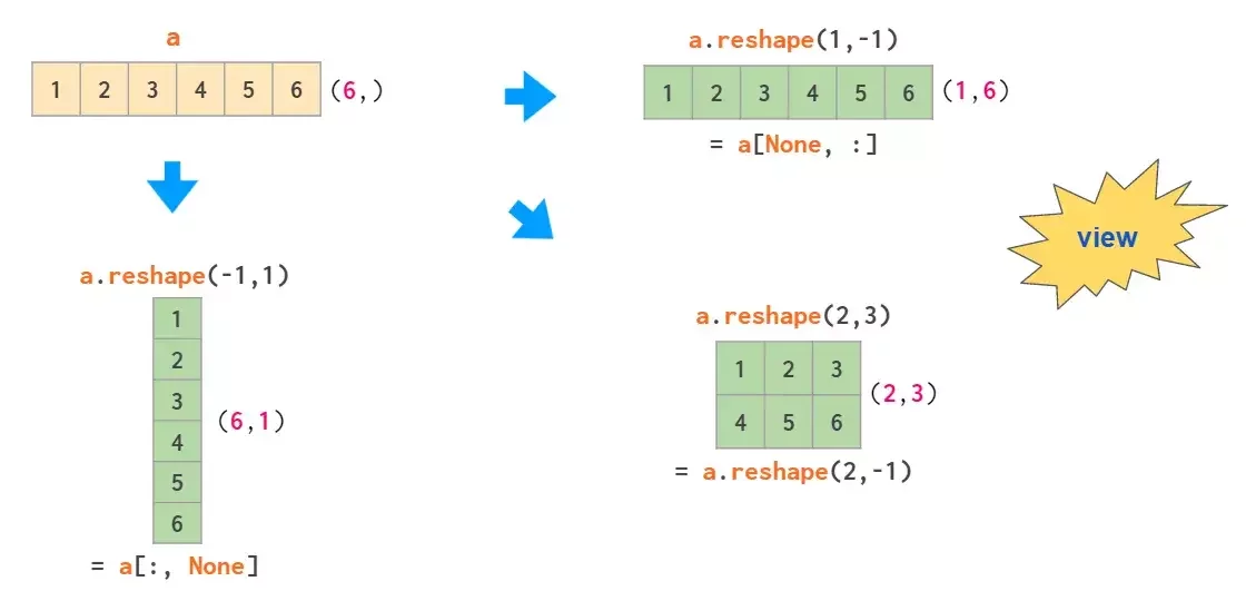
a.reshape(2,3)Creating Matrices from Arrays
When you have a single, long array and you want to turn it into a matrix:
Go back with the flatten() method!
a.flatten()Row and Column Vectors
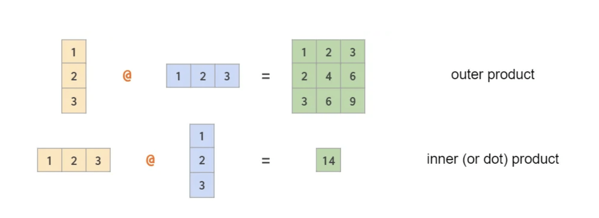
You can use the @ operator to perform dot/outer products on 2 vectors
But how does numpy know if the vector is a row vector or a column vector?
We must encode the 1D vectors as 2D vectors
(3,1) @ (1,3) -> (3x3)
(1,3) @ (3,1) -> (1x1)
Row and Column Vectors
np.array([1, 2, 3, 4])Normal 1D Vector (4,)
4 rows, 0 columns
np.array([[1, 2, 3, 4]])Row 2D Vector (1, 4)
1 row, 4 columns
np.array([[1], [2], [3], [4]])Column 2D Vector (4, 1)
4 rows, 1 column
Notice how this has double brackets, making it a 2D matrix with 1 row!
Row and Column Vectors
np.array([1, 2, 3, 4])Normal 1D Vector (4,)
4 rows, 0 columns
np.array([[1, 2, 3, 4]])Row 2D Vector (1, 4)
1 row, 4 columns
np.array([[1], [2], [3], [4]])Column 2D Vector (4, 1)
4 rows, 1 column
x.Tx.Tx.reshape(1, -1)x.flatten()x.reshape(-1, 1)x.flatten()Challenge #5
Challenge #5
Let's play around with tensors:
- Initialize a size (2,3,4) tensor with random integers between 0-9
- Print the tensor and examine what it looks like
- Check its .shape attribute
- Transpose the matrix. Print it. What is the shape?
- Try to .flatten() the matrix. What does it look like now? What is the shape?
- Try to reshape the flattened version back to its original (2,3,4) tensor
One last (useful) thing!
Saving and loading numpy arrays
- You can save a numpy array to a file
- Great for backing up you work!
import numpy as np

a = np.arange(6).reshape(2,3)

np.save("my_array.npy", a)   # save to file
b = np.load("my_array.npy")  # load back

print(b)
print(f"They are equal: {np.all(a == b)}")
Surprise mini-challenge:
Why did I use np.all() in the above code
Lecture 4
- Recap
- Project Scaffolding with uv
- Python Notebooks
- Linear Algebra in a Nutshell
- NumPy Fundamentals
The End
Learning Data Science Lecture 4
By astrojarred
Private


