Learning Data Science
Lecture 5
Visualisation Craft
Project Scaffolding
- Starting projects with uv
- Adding your local project to GitHub
- Installing external packages
uv init -p 3.13uv add numpy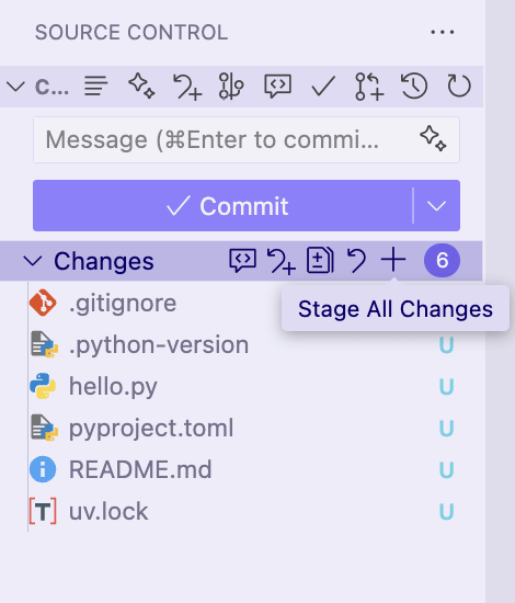
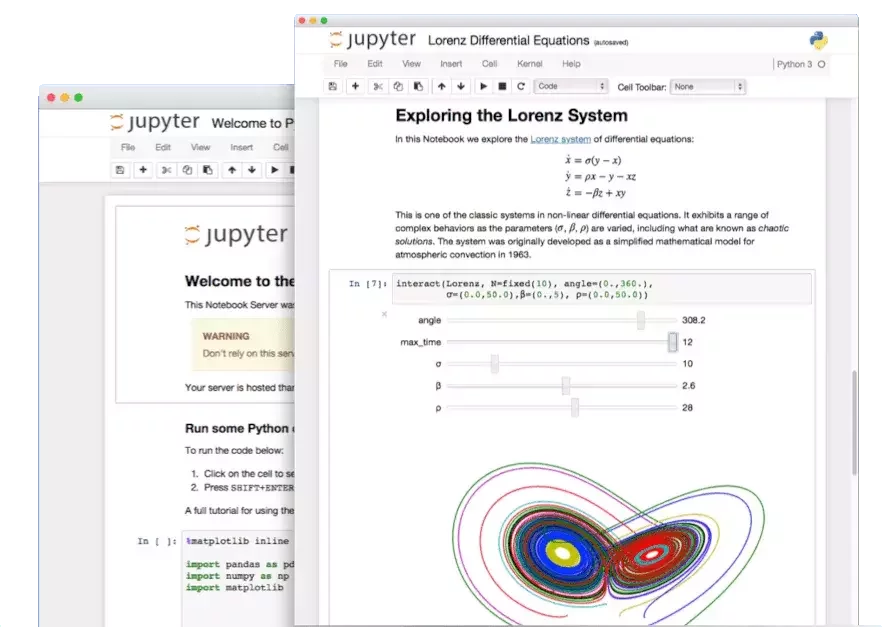
Python Notebooks
Ways to interact with Python code
REPL
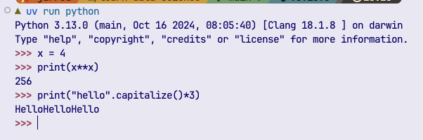
✅ Interactive
❌ Sharable
❌ Version Control friendly
❌ Reproducible
❌ Mix code, text, plots
Scripts
❌ Interactive
✅ Sharable
✅ Version Control friendly
✅ Reproducible
❌ Mix code, text, plots
Notebooks
✅ Interactive
✅ Sharable
⚠️ Version Control friendly
⚠️ Reproducible
✅ Mix code, text, plots
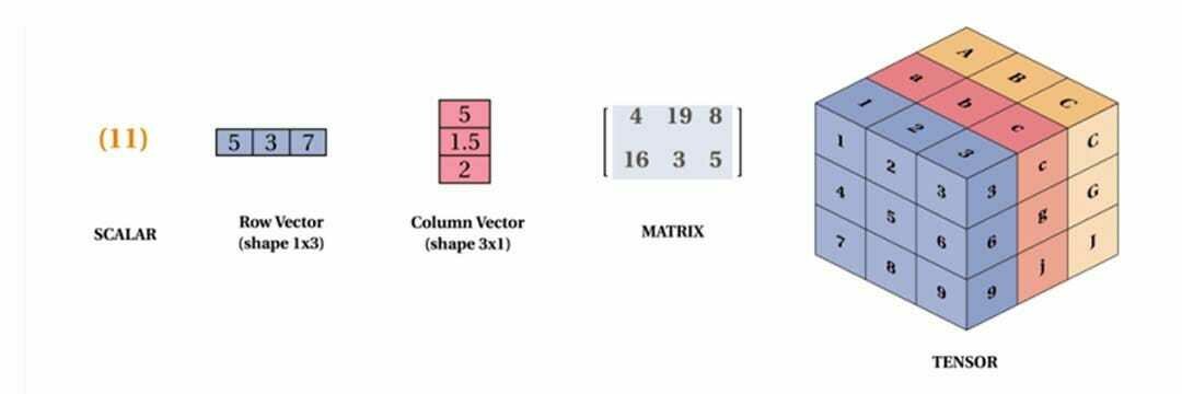
Linear Algebra in a Nutshell
The math of vectors and matrices
How to combine and transform them
Everything is a tensor
Graphics from: St. Lawrence U CS140 and Montesinos-López et al (2022)
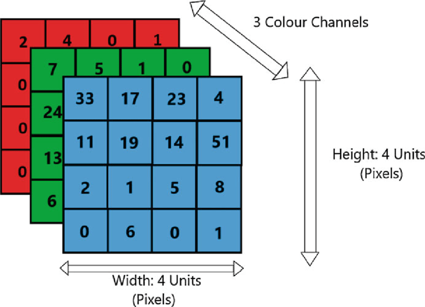
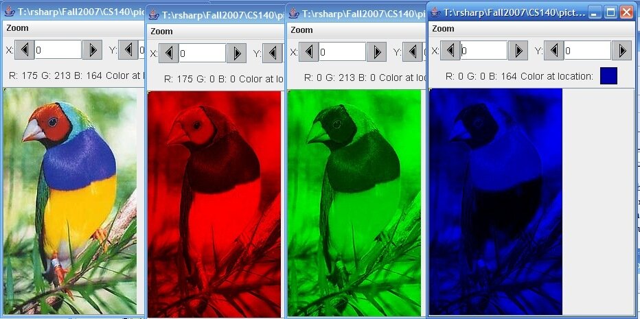
Image width (4px)
Image height (4px)
Image "depth"
(3 color channels)
NumPy
an array library that powers all of scientific Python
Fancy lists
Vectors
Matrices
Tensors
x = np.array([1,2,3,4,5])
# OR
l = [1, 2, 3, 4, 5]
x = np.array(l)
x = np.ones(5)
x = np.zeros(5)x = np.array([1,2,3,4,5])
y = np.ones_like(x)x = np.arange(6)
x = np.arange(1, 6, 2)
x = np.linspace(0, 1, 11)rng = np.random.default_rng()
# 5 ints between [0,100)
rng.integers(0, 100, 5)
# 10 ints between [0, 1)
rng.random(10)
# 6 samples from a gaussian
# mean=5, std=3
rng.normal(5, 3, 6)x = np.arange(1, 6)
# [1, 2, 3, 4, 5]
x[1] # = 2
x[2:4] # = [3, 4]
# everything from index -2 and onwards
x[-2:] # = [4, 5]
# Every 2 indices (step=2)
x[::2] # = [1, 3, 5]
# specifically indicies 1, 3, 4
x[[1, 3, 4]] # = [2, 4, 5]x = np.array([1, 2])
y = np.array([3, 6])
x + y # = [4, 8]
x * y # = [3, 12]
x + 2 # = [3, 4]
np.sqrt(x)
np.sin(x)x.max()
x.sum()
x.mean()
# etcnp.array([1, 2, 3, 4])Normal 1D Vector (4,)
4 rows, 0 columns
np.array([[1, 2, 3, 4]])Row 2D Vector (1, 4)
1 row, 4 columns
np.array([[1], [2], [3], [4]])Column 2D Vector (4, 1)
4 rows, 1 column
x.Tx.Tx.reshape(1, -1)x.flatten()x.reshape(-1, 1)x.flatten()Lecture 5
- Recap
- Why visualization
- Matplotlib essentials
- Seaborn quick tour
- Important file formats
Why Visualize Anything?
- Sight is often regarded as the dominant sense
- Sight is often claimed to be the most "objective" sense
Debatable!
Clearly not true for everyone!
However, we use our sight often to better understand scientific results:
- Reading journals and textbooks
- Looking at slides
- Looking at graphs

Listening to data
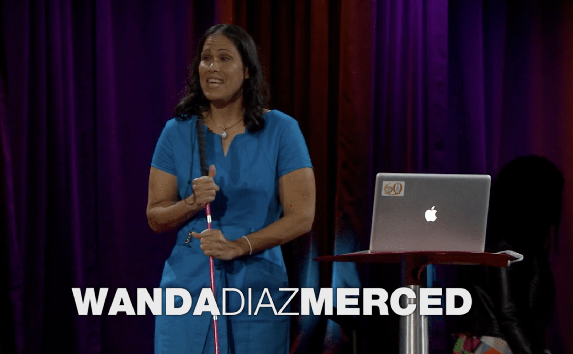
"When we synchronize our different ways of perceiving the world, our sensitivity to events that are masked to the eye ... increases exponentially."
Listening to data
While today we're going to talk about visual ways to communicate data, always remember there are other ways too!
Why Visualization?
[[-0.99582463  0.99785717]
 [-0.98329854  0.9975254 ]
 [-0.97077244  0.99820004]
 [-0.95824635  0.99651706]
 [-0.94572025  0.99664487]
 [-0.93319415  0.99538239]
 [-0.92066806  0.995524  ]
 [-0.90814196  0.99469056]
 [-0.89561587  0.99384034]
 [-0.88308977  0.99323822]
 [-0.87056367  0.99233328]
 [-0.85803758  0.99210751]
 [-0.84551148  0.99107832]
 [-0.83298539  0.99010279]
 [-0.82045929  0.98942019]
 [-0.80793319  0.98934844]
 [-0.7954071   0.98927283]
 [-0.782881    0.98808468]
 [-0.77035491  0.98737426]
 [-0.75782881  0.98696232]
 [-0.74530271  0.98682547]
 [-0.73277662  0.98587808]
 [-0.72025052  0.98514856]
 [-0.70772443  0.98531636]
 [-0.69519833  0.98464728]
 [-0.68267223  0.9847355 ]
 [-0.67014614  0.98388559]
 [-0.65762004  0.98306121]
 [-0.64509395  0.98279164]
 [-0.63256785  0.98383771]
 [-0.62004175  0.98375677]
 [-0.60751566  0.98293767]
 [-0.59498956  0.98383009]
 [-0.58246347  0.98452698]
 [-0.56993737  0.98345948]
 [-0.55741127  0.98350519]
 [-0.54488518  0.98408205]
 [-0.53235908  0.9836294 ]
 [-0.51983299  0.98374858]
 [-0.50730689  0.98364951]
 [-0.49478079  0.98381505]
 [-0.4822547   0.98420902]
 [-0.4697286   0.98364914]
 [-0.45720251  0.98383823]
 [-0.44467641  0.9827292 ]
 [-0.43215031  0.98349927]
 [-0.41962422  0.98315183]
 [-0.40709812  0.98297283]
 [-0.39457203  0.9830812 ]
 [-0.38204593  0.98327179]
 [-0.36951983  0.98374565]
 [-0.35699374  0.98282346]
 [-0.34446764  0.98334186]
 [-0.33194154  0.9831124 ]
 [-0.31941545  0.98315234]
 [-0.30688935  0.98366272]
 [-0.29436326  0.98345594]
 [-0.28183716  0.9837556 ]
 [-0.26931106  0.98313967]
 [-0.25678497  0.98290479]
 [-0.24425887  0.98307619]
 [-0.23173278  0.98324617]
 [-0.21920668  0.98320411]
 [-0.20668058  0.9826849 ]
 [-0.19415449  0.98314091]
 [-0.18162839  0.98318293]
 [-0.1691023   0.98408642]
 [-0.1565762   0.98381884]
 [-0.1440501   0.98271634]
 [-0.13152401  0.9829331 ]
 [-0.11899791  0.98245396]
 [-0.10647182  0.98279521]
 [-0.09394572  0.98315076]
 [-0.08141962  0.98350076]
 [-0.06889353  0.98272155]
 [-0.05636743  0.98274717]
 [-0.04384134  0.98214642]
 [-0.03131524  0.98293766]
 [-0.01878914  0.98257601]
 [-0.00626305  0.98278833]
 [ 0.00626305  0.98264936]
 [ 0.01878914  0.98296328]
 [ 0.03131524  0.98229963]
 [ 0.04384134  0.98241852]
 [ 0.05636743  0.98386052]
 [ 0.06889353  0.98249822]
 [ 0.08141962  0.9825797 ]
 [ 0.09394572  0.98375928]
 [ 0.10647182  0.98419352]
 [ 0.11899791  0.98257071]
 [ 0.13152401  0.98290075]
 [ 0.1440501   0.98319426]
 [ 0.1565762   0.98375958]
 [ 0.1691023   0.98268469]
 [ 0.18162839  0.98299352]
 [ 0.19415449  0.98341565]
 [ 0.20668058  0.98329256]
 [ 0.21920668  0.98298301]
 [ 0.23173278  0.98309564]
 [ 0.24425887  0.98261577]
 [ 0.25678497  0.98308789]
 [ 0.26931106  0.98309491]
 [ 0.28183716  0.98331351]
 [ 0.29436326  0.98301856]
 [ 0.30688935  0.98345023]
 [ 0.31941545  0.98368849]
 [ 0.33194154  0.98336824]
 [ 0.34446764  0.98347031]
 [ 0.35699374  0.98337527]
 [ 0.36951983  0.98337933]
 [ 0.38204593  0.98311682]
 [ 0.39457203  0.98355906]
 [ 0.40709812  0.98342144]
 [ 0.41962422  0.98432639]
 [ 0.43215031  0.9841481 ]
 [ 0.44467641  0.98370361]
 [ 0.45720251  0.98327543]
 [ 0.4697286   0.98316794]
 [ 0.4822547   0.98412248]
 [ 0.49478079  0.98378512]
 [ 0.50730689  0.98390695]
 [ 0.51983299  0.98305279]
 [ 0.53235908  0.98415821]
 [ 0.54488518  0.98400649]
 [ 0.55741127  0.9834189 ]
 [ 0.56993737  0.98371369]
 [ 0.58246347  0.98404789]
 [ 0.59498956  0.98400435]
 [ 0.60751566  0.98289261]
 [ 0.62004175  0.98302591]
 [ 0.63256785  0.98307655]
 [ 0.64509395  0.98339993]
 [ 0.65762004  0.98413959]
 [ 0.67014614  0.98278563]
 [ 0.68267223  0.98402645]
 [ 0.69519833  0.98454638]
 [ 0.70772443  0.98499224]
 [ 0.72025052  0.98516417]
 [ 0.73277662  0.98508764]
 [ 0.74530271  0.98643427]
 [ 0.75782881  0.98753893]
 [ 0.77035491  0.98680817]
 [ 0.782881    0.98836621]
 [ 0.7954071   0.98850978]
 [ 0.80793319  0.98925487]
 [ 0.82045929  0.9895102 ]
 [ 0.83298539  0.99045925]
 [ 0.84551148  0.99178033]
 [ 0.85803758  0.99216214]
 [ 0.87056367  0.99328812]
 [ 0.88308977  0.99372549]
 [ 0.89561587  0.99407863]
 [ 0.90814196  0.99523416]
 [ 0.92066806  0.99532697]
 [ 0.93319415  0.99607476]
 [ 0.94572025  0.99619085]
 [ 0.95824635  0.99687223]
 [ 0.97077244  0.99706969]
 [ 0.98329854  0.99821132]
 [ 0.99582463  0.9977719 ]]
Why Visualization?
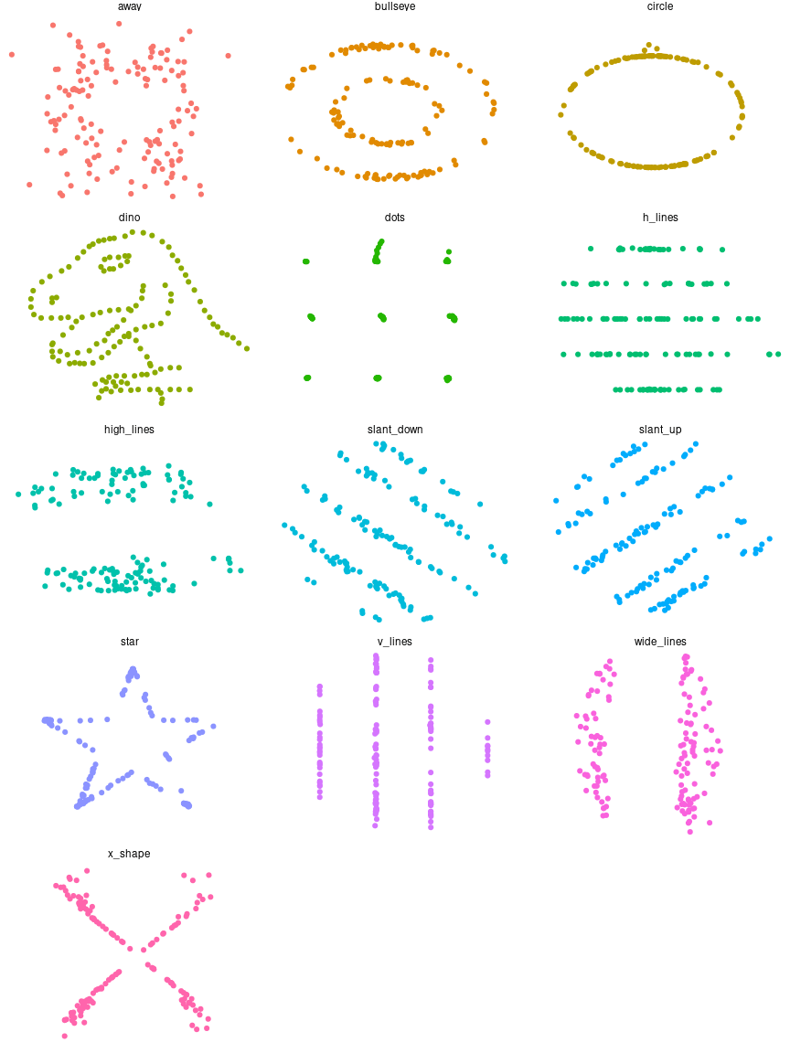

Alberto Cairo’s "Datasaurus Dozen"
- Distributions with the exact same statistics
- But visually completely different!
Looking at the numbers alone is not enough!
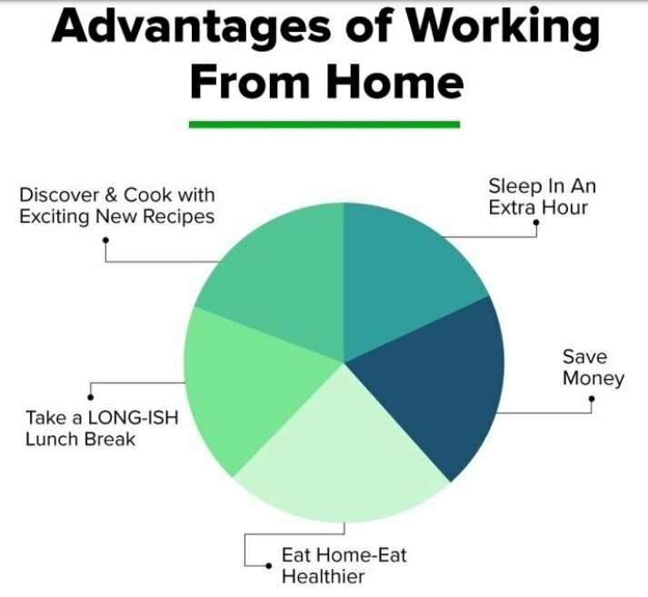
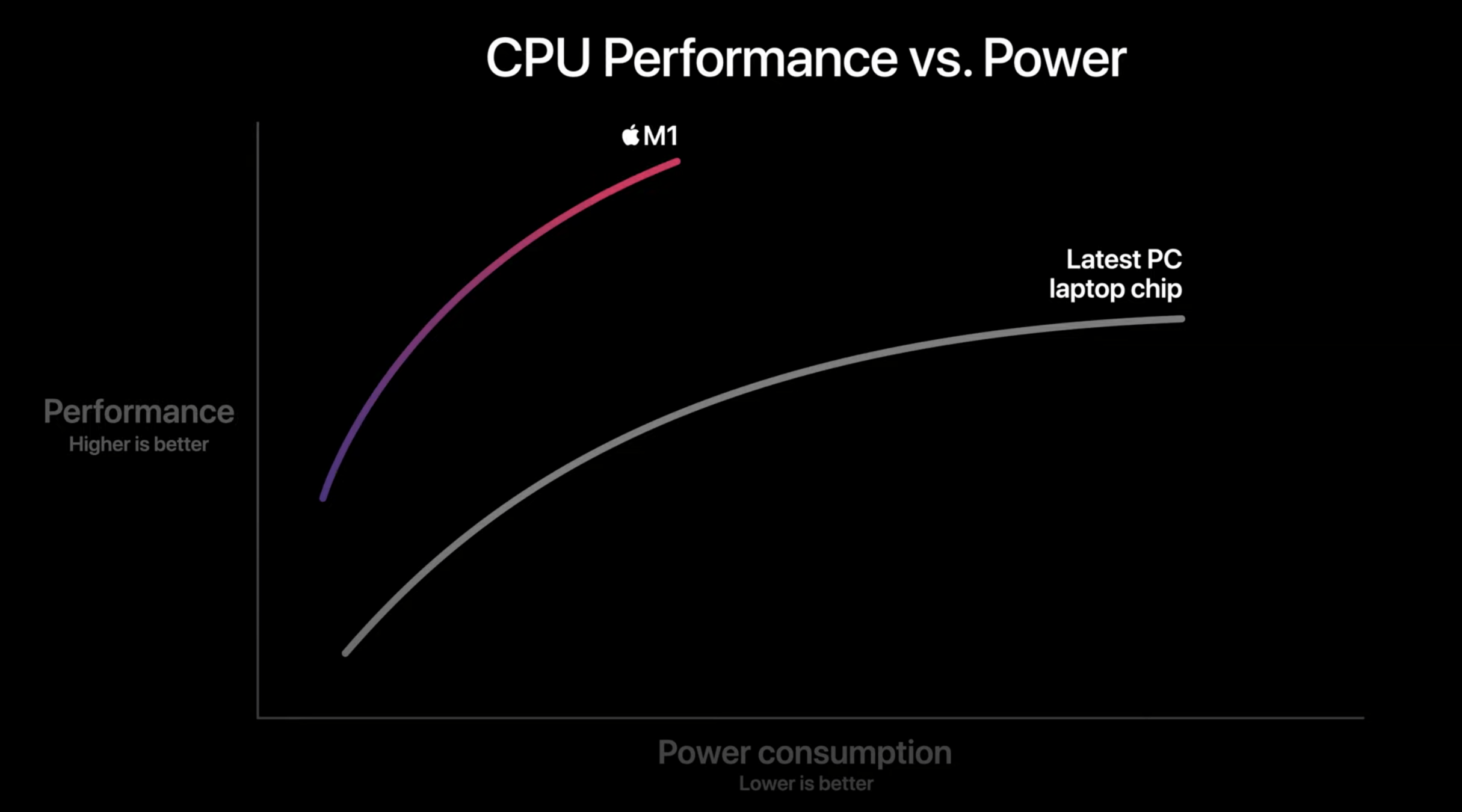
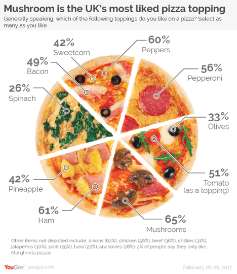
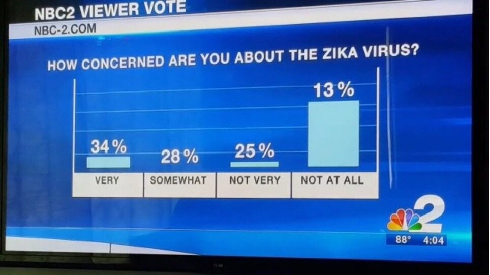
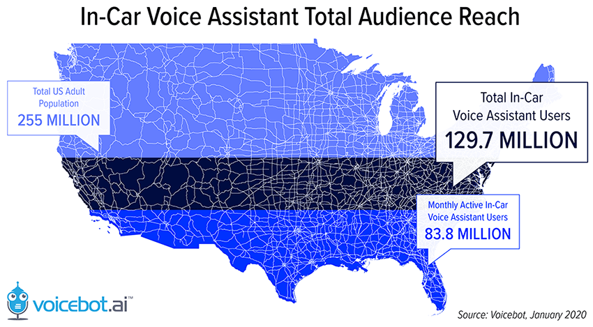
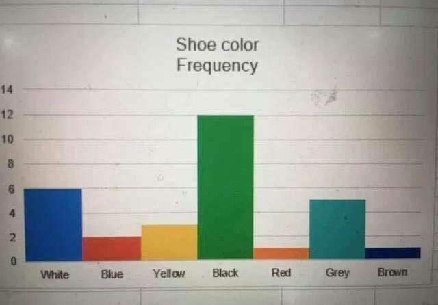
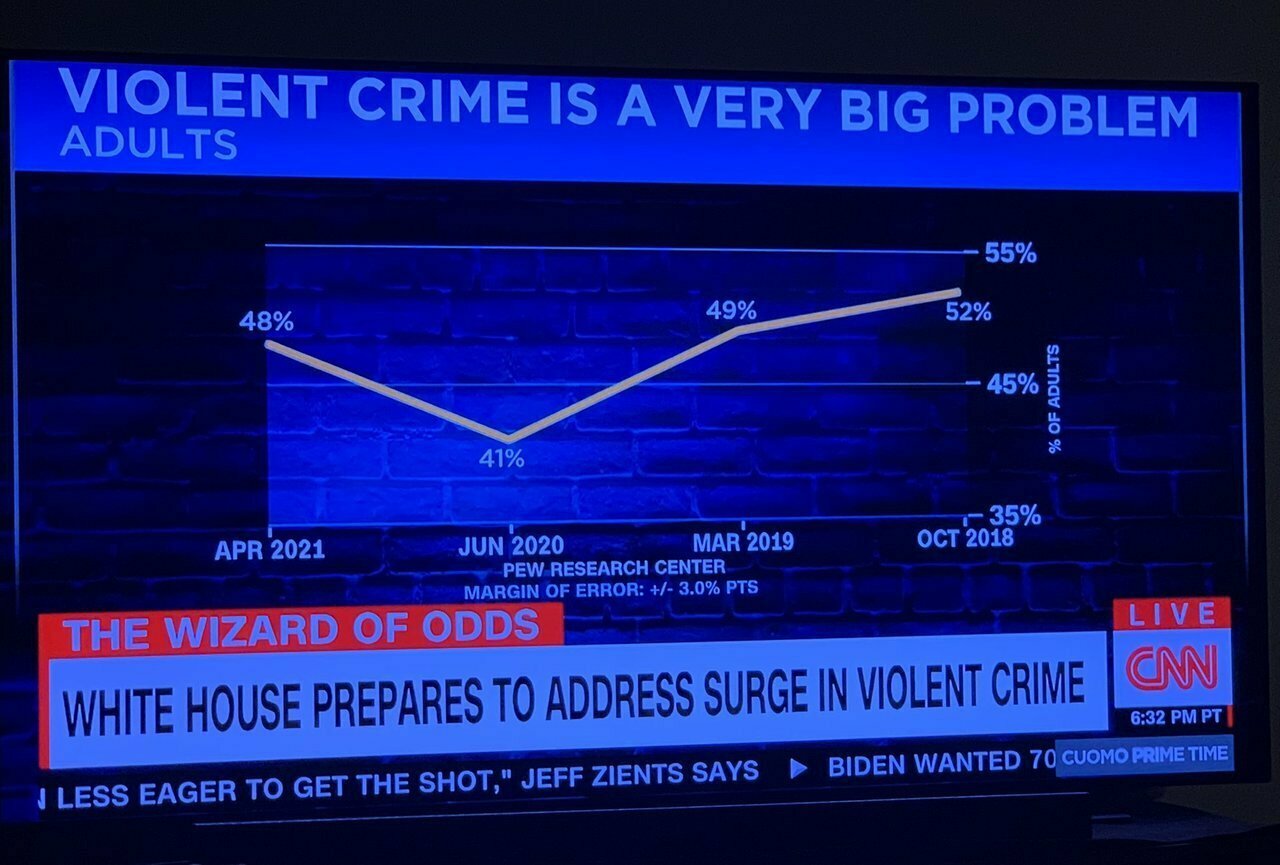
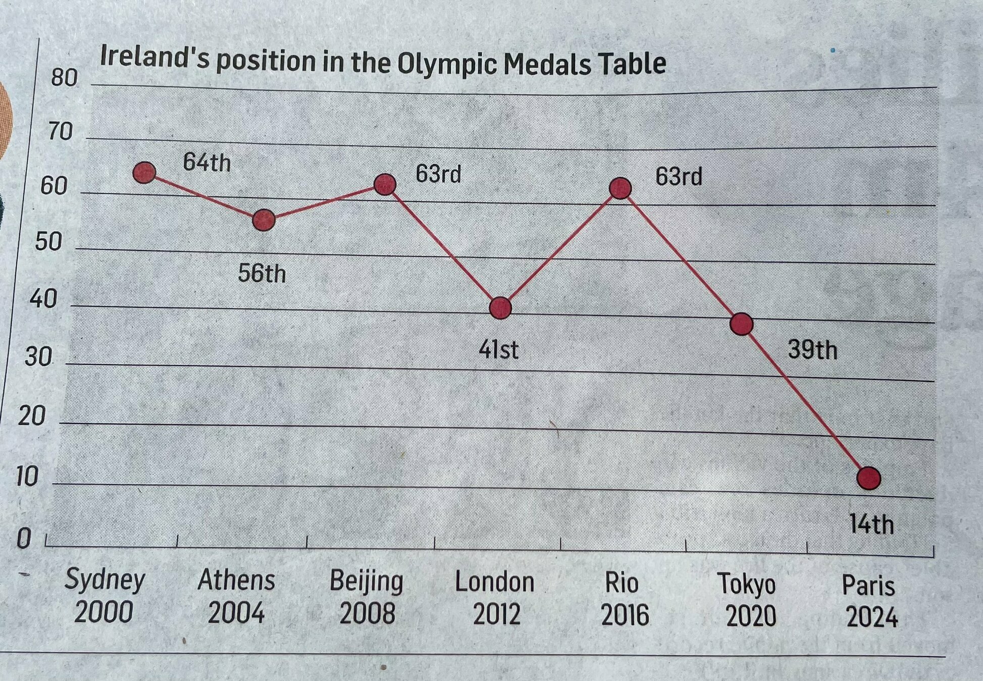
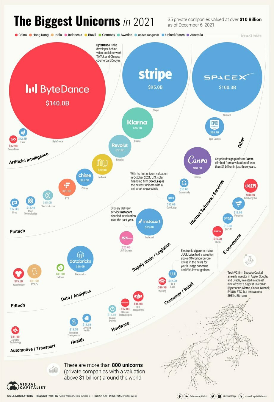
Challenge #1
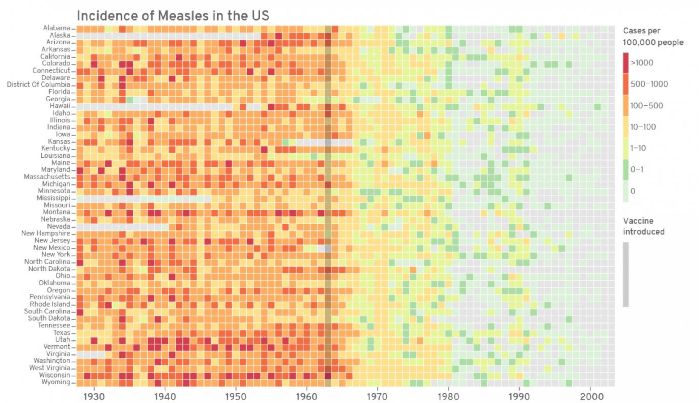
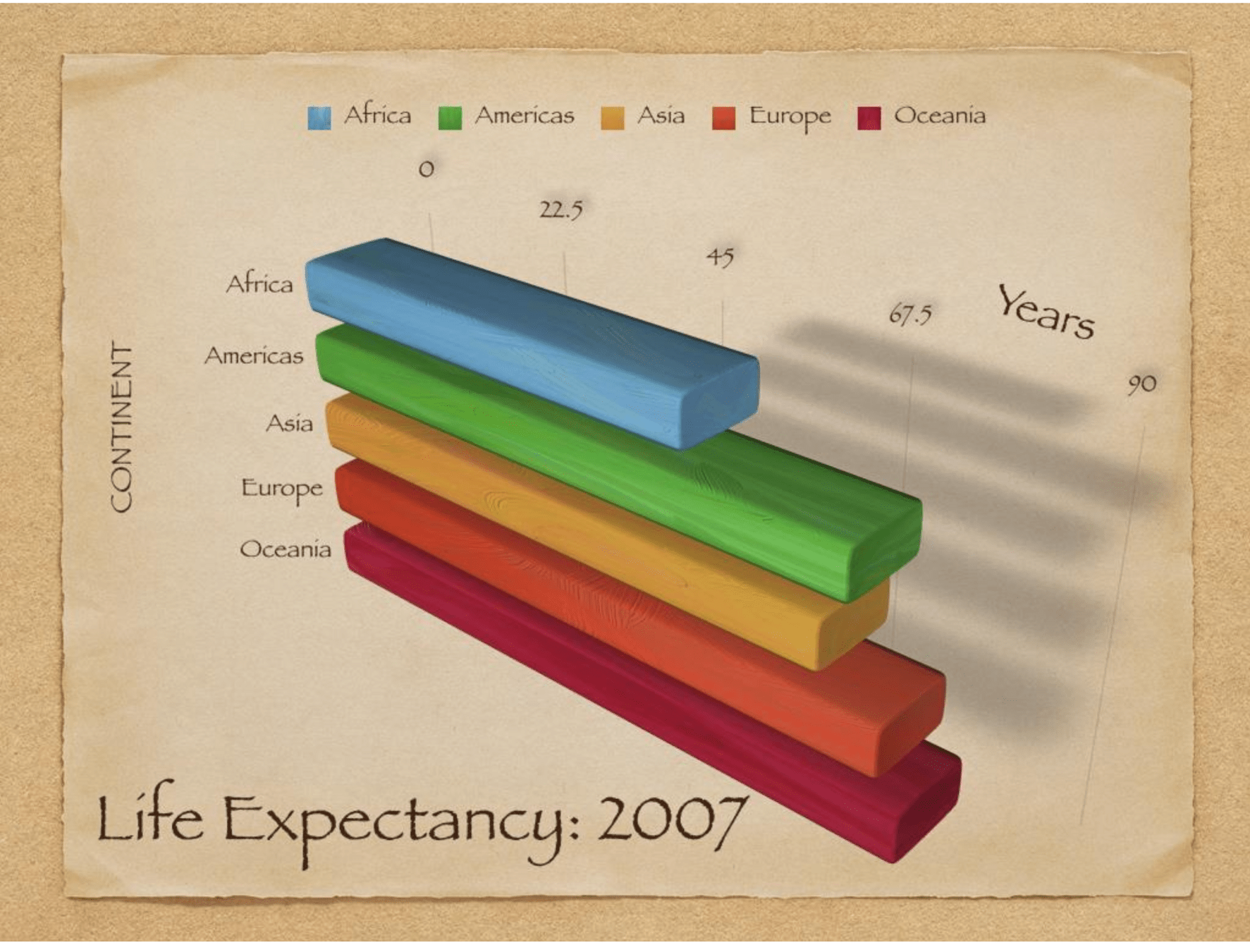
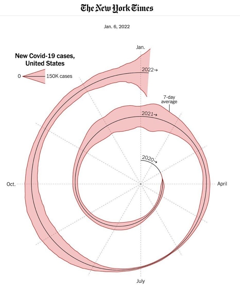
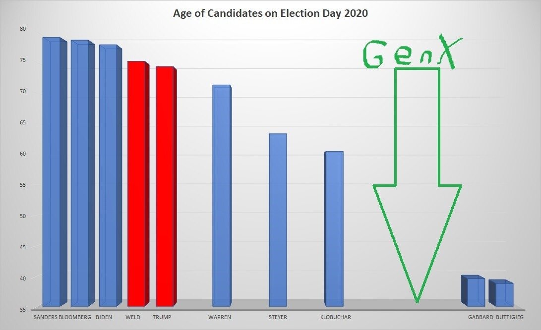
Find what is off, weird, confusing, misleading, or 'too much' in each of the following visualizations:

Previous president of Colombia claiming that collective homicides went down during his time in office (2018-2020)
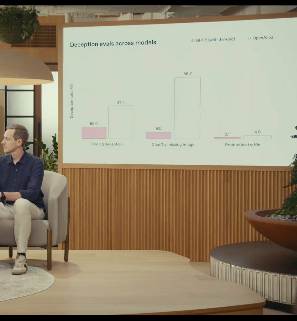
Open AI's Official
ChatGPT 5 Release Video
(Aug 2025)
Lecture 5
- Recap
- Why visualization
- Matplotlib essentials
- Seaborn quick tour
- Important file formats
matplotlib
Create visualizations:
- static
- animated
- interactive
Generally flexible enough to do whatever you need

Installing matplotlib
uv add matplotlibimport matplotlib.pyplot as pltImporting matplotlib
Everyone nicknames this package to plt!
Plotting Functions with line plots
Making Plots
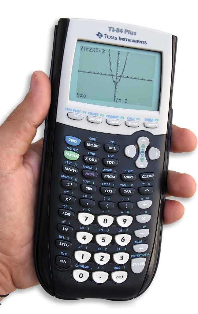
x = np.array([-5, -4, -3, -2, -1, 0, 1, 2, 3, 4, 5])

y = [i**2 for i in x]

plt.plot(x, y)
plt.show()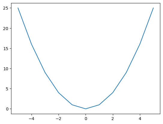
Making Plots
x = np.linspace(-10, 10, 1000)
y = [i**2 for i in x]

plt.plot(x, y)
plt.show()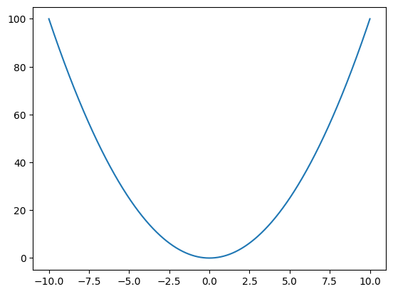
- Make the plot even smoothing by plotting 1000 points inside our range
- Recall linspace is similar to the builtin range function
Add title and axis labels
x = np.linspace(-10, 10, 1000)
y = [i**2 for i in x]

plt.plot(x, y)

plt.title("A plot of $f(x) = x^2$")
plt.xlabel("x")
plt.ylabel("$x^2$")

plt.show()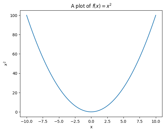
- Tip: if you know how to write latex math, this also works inside plots!
Scatter Plot
Scatter Plot
rng = np.random.default_rng()

x = rng.normal(0, 1, 20)
y = rng.normal(0, 1, 20)

plt.scatter(x, y)
plt.show()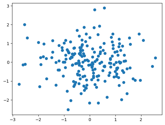
Good for unordered, 2D data
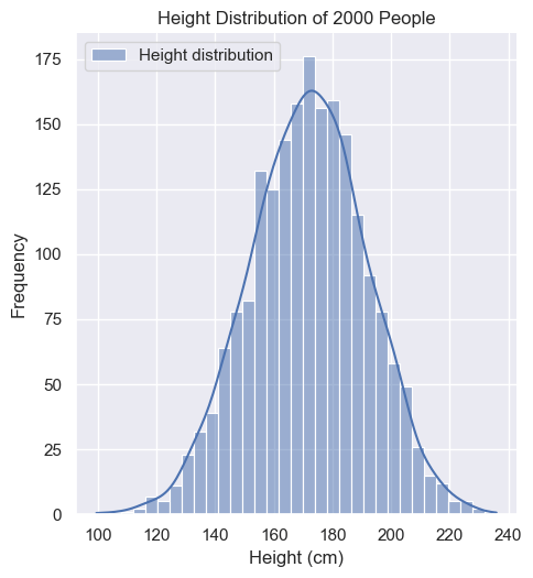
Histograms
Histograms
x = rng.normal(171, 20, 2000)

plt.hist(x)
plt.xlabel("Height (cm)")
plt.ylabel("Frequency")
plt.title("Height Distribution of 2000 People")
plt.show()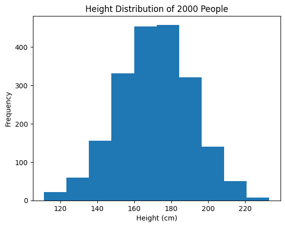
Show the frequency distribution of 1D data
Axes and Labels
Axes and Labels
rng = np.random.default_rng()

x = rng.normal(0, 1, 20)
y = rng.normal(0, 1, 20)

plt.scatter(x, y)
plt.show()
Same scatter as before
Axes and Labels
rng = np.random.default_rng()

x = rng.normal(0, 1, 200)
y = rng.normal(0, 1, 200)

plt.scatter(x, y)
plt.xlabel("X-axis")
plt.ylabel("Y-axis")
plt.title("My Great Scatter Plot")
plt.show()
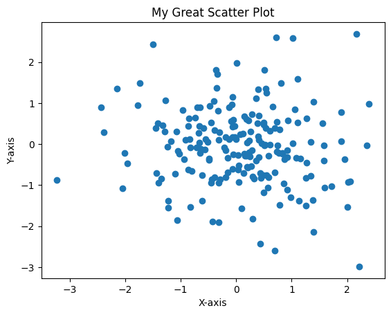
Can set x and y axes, as well as title
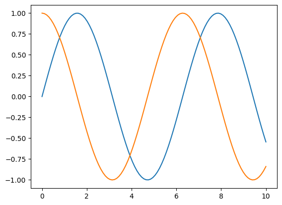
Overplotting and Legends
x = np.linspace(0, 10, 100)
y1 = np.sin(x)
y2 = np.cos(x)

plt.plot(x, y1)
plt.plot(x, y2)
plt.show()
Anything you do before 'show()' will all show up on the same axes!
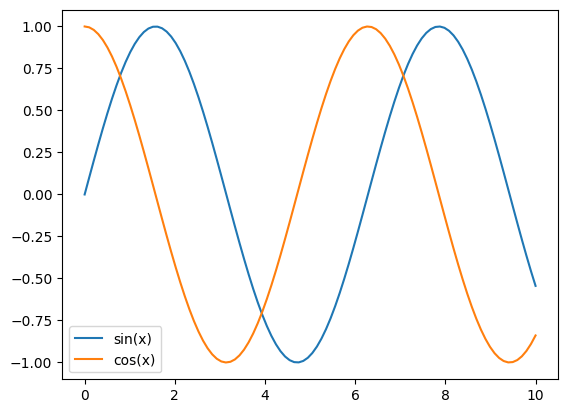
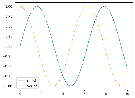
Overplotting and Legends
x = np.linspace(0, 10, 100)
y1 = np.sin(x)
y2 = np.cos(x)

plt.plot(x, y1, label="sin(x)")
plt.plot(x, y2, label="cos(x)")
plt.legend()
plt.show()
Use the 'label' kwarg, and add plt.legend() to automatically make a Legend!
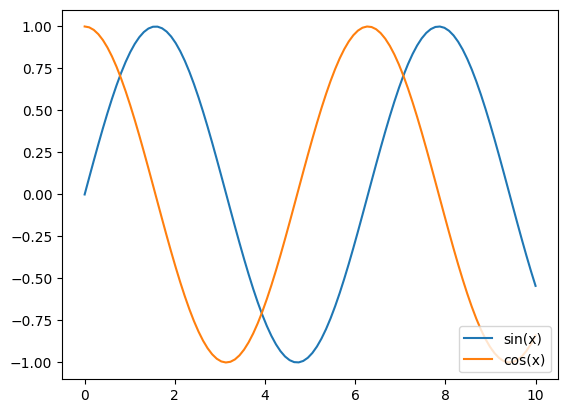
Overplotting and Legends
x = np.linspace(0, 10, 100)
y1 = np.sin(x)
y2 = np.cos(x)
plt.plot(x, y1, label="sin(x)")
plt.plot(x, y2, label="cos(x)")
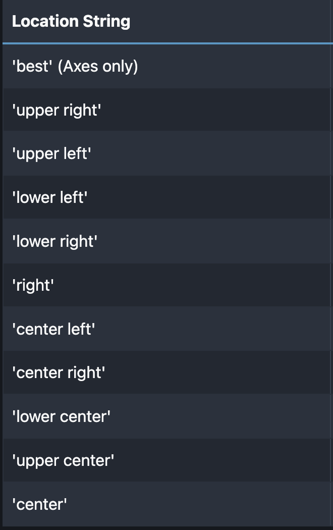
plt.legend(loc="lower right")
plt.show()Use the loc kwarg to select the position of the legend!
Overplotting and Legends
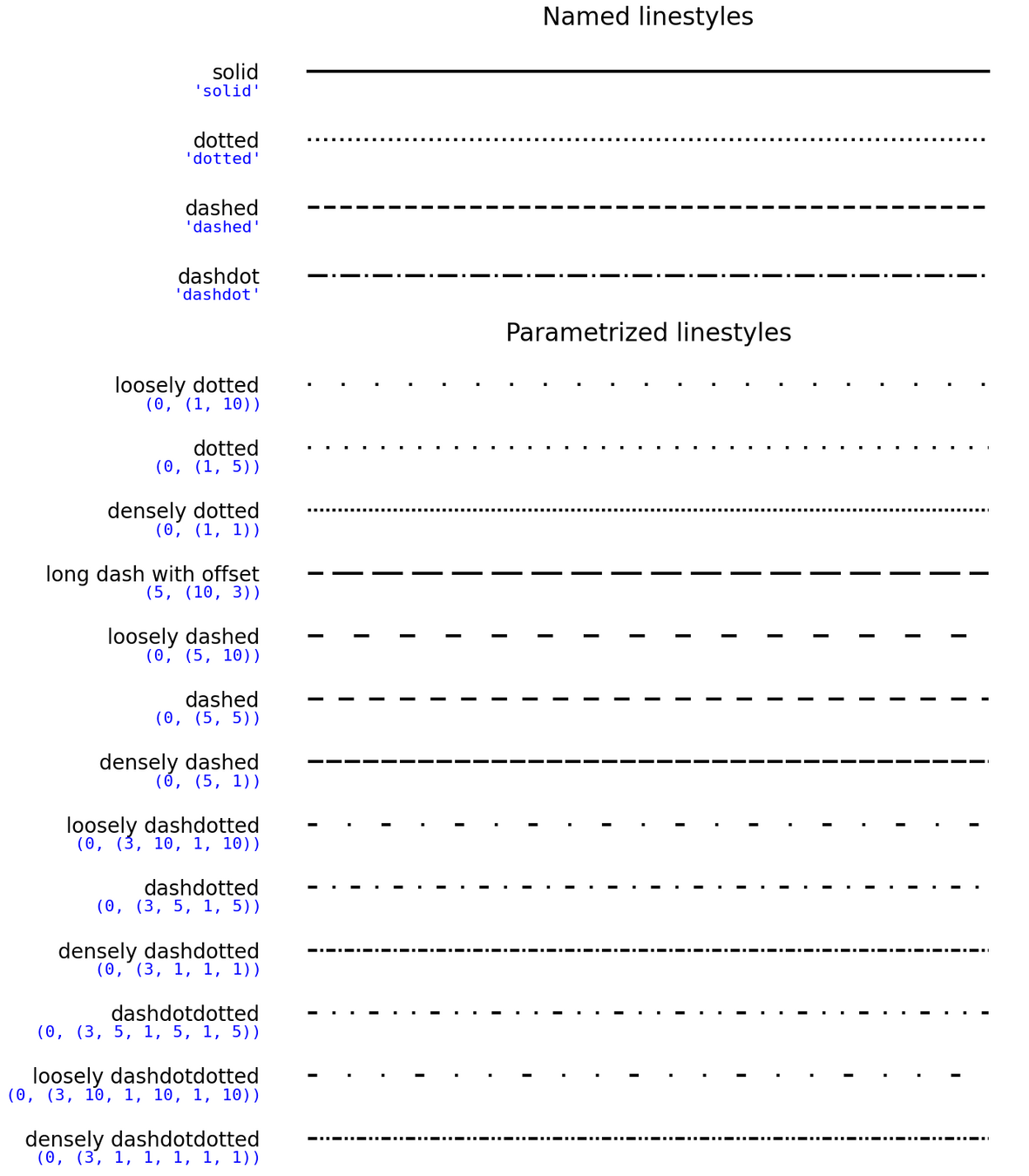
Style
Style
- Line style
- Marker Style
- Color
- Width
- Alpha
Line Style
y1 = np.sin(x)
y2 = np.cos(x)

plt.plot(x, y1, label="sin(x)", linestyle="dashed")
plt.plot(x, y2, label="cos(x)", linestyle="dotted")
plt.legend()
plt.show()
Use the loc kwarg to select the position of the legend!
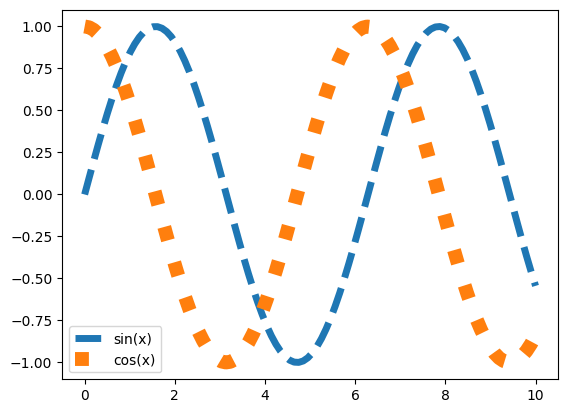
Line Style
Line Style
plt.plot(x, y1, label="sin(x)", linewidth=5, linestyle="dashed")
plt.plot(x, y2, label="cos(x)", linewidth=10, linestyle="dotted")
plt.legend()
plt.show()
Change the width of your lines
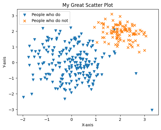
Marker Style
plt.scatter(x, y, marker="v", label="People who do", )
plt.scatter(x2, y2, marker="x", label="People who do not", )
plt.xlabel("X-axis")
plt.ylabel("Y-axis")
plt.title("My Great Scatter Plot")
plt.legend()
plt.show()
Change the shape of points:
full list here
Marker Style
plt.scatter(x, y, marker="v", label="People who do", )
plt.scatter(x2, y2, marker="x", label="People who do not", )
plt.xlabel("X-axis")
plt.ylabel("Y-axis")
plt.title("My Great Scatter Plot")
plt.legend()
plt.show()
Change the size of the markers
Color
New overplots automatically cycle through a list of colors
Color
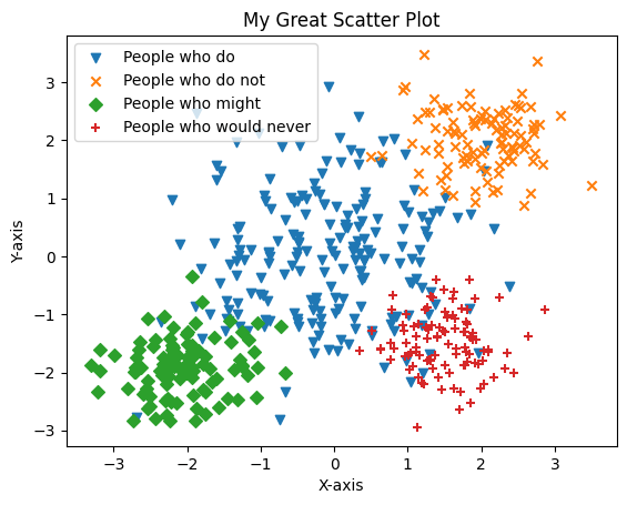
You can also set the colors you want specifically.
plt.scatter(x, y, color="red", label="People who do", marker="v")
plt.scatter(x2, y2, color="blue", label="People who do not", marker="x")
plt.scatter(x3, y3, color="green", label="People who might", marker="D")
plt.scatter(x4, y4, color="#6f42c1", label="People who would never", marker="+")
plt.xlabel("X-axis")
plt.ylabel("Y-axis")
plt.title("My Great Scatter Plot")
plt.legend()
plt.show()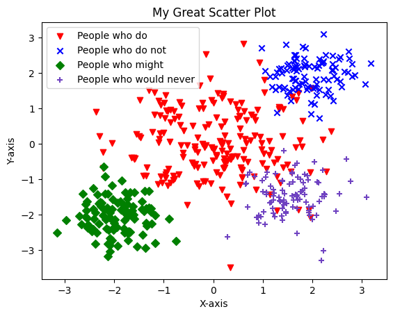
Marker Size
Use the 's' variable,
represented in area^2 of the plot
plt.scatter(x, y, s=5, label="People who do", marker="v")
plt.scatter(x2, y2, s=100, label="People who do not", marker="x")
plt.xlabel("X-axis")
plt.ylabel("Y-axis")
plt.title("My Great Scatter Plot")
plt.legend()
plt.show()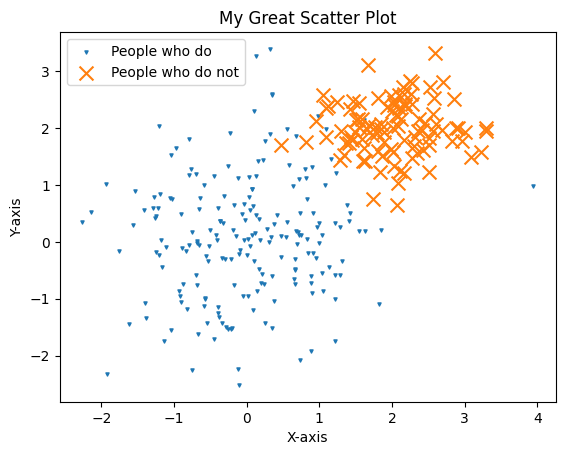
Alpha (Transparency)
Change the opacity of curves/markers. Alpha is in the range [0,1]
plt.plot(x, y1, alpha=0.9, color="#5a2094")
plt.plot(x, y2, alpha=0.8, color="#5a2094")
plt.plot(x, y3, alpha=0.5, color="#5a2094")
plt.plot(x, y4, alpha=0.3, color="#5a2094")
plt.plot(x, y5, alpha=0.1, color="#5a2094")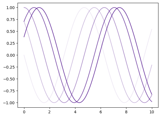
Log Scale
Log Scale
x = np.linspace(0, 100, 1000)
y = np.exp(x)

plt.plot(x, y)
plt.xlabel("X-axis")
plt.ylabel("Y-axis")
plt.title("Normal Axes")
plt.show()

plt.plot(x, y)
plt.yscale("log")
plt.xlabel("X-axis")
plt.ylabel("Y-axis")
plt.title("Logarithmic Axes")
plt.show()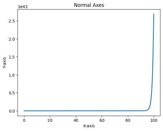
Log Scale
x = np.linspace(0, 100, 1000)
y = np.exp(x)

plt.plot(x, y)
plt.xlabel("X-axis")
plt.ylabel("Y-axis")
plt.title("Normal Axes")
plt.show()

plt.plot(x, y)
plt.yscale("log")
plt.xlabel("X-axis")
plt.ylabel("Y-axis")
plt.title("Logarithmic Axes")
plt.show()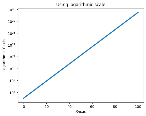
Use plt.xscale or plt.yscale
Saving Plots
Saving Plots
Can always drag out of a notebook
Saving Plots
Can also save the file from code
- Just add the plt.savefig() name
- Can export to many different file types
- Just change the suffix at the end of "my_plot.png" to match the filet ype you wanted
x = np.linspace(-10, 10, 1000)
y = [i**2 for i in x]

plt.plot(x, y)

plt.title("A plot of $f(x) = x^2$")
plt.xlabel("x")
plt.ylabel("$x^2$")
plt.savefig("my_plot.png")
plt.show()
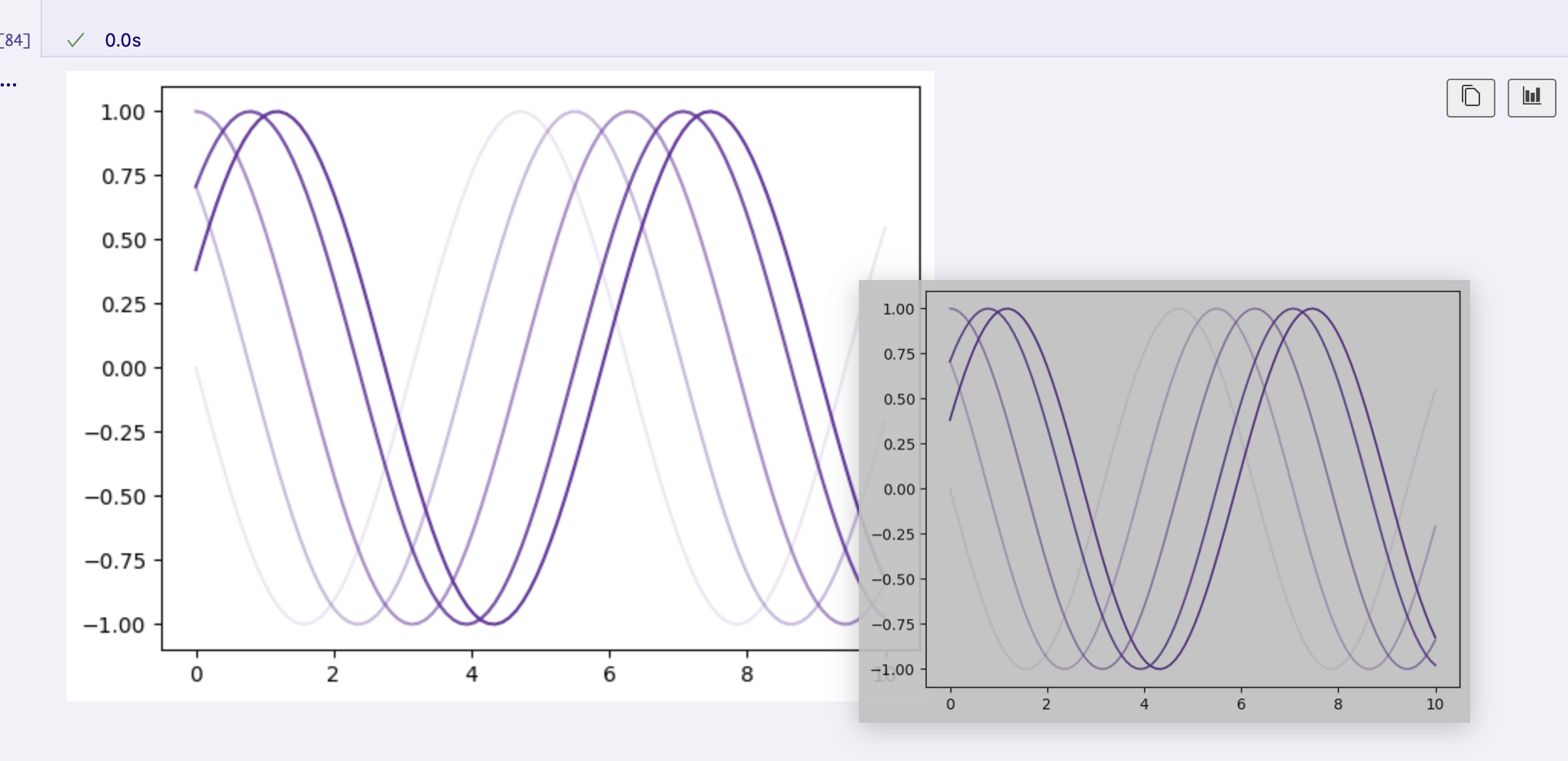
Challenge #1
Challenge #1
Try to recreate this figure as exact as possible!
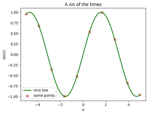
Figure Size
Figure Size
plt.figure(figsize=(10, 5))
plt.plot(x, y)
plt.show()

plt.figure(figsize=(3, 10))
plt.plot(x, y)
plt.show()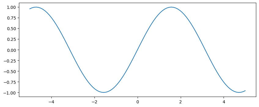
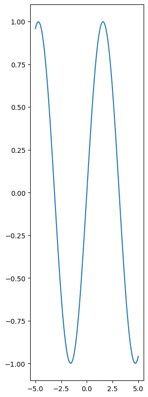
plt.figure(figsize=(X,Y))
💫 You are now a master plot maker!
If you're someone who likes design, you might have noticed they are not so pretty by default.
Let's look at a tool which can help 💅
Lecture 5
- Recap
- Why visualization
- Matplotlib essentials
- Seaborn quick tour
- Important file formats
What is seaborn?
Seaborn is a library built on top of matplotlib
Attempts to make your plots
✨effortlessly pretty✨
just like you
ALSO: Provides a user-friendly high-level interface for making statistical plots
What is seaborn?
Installing seaborn
uv add seabornimport seaborn as snsStarting seaborn
import matplotlib.pyplot as plt
import seaborn as sns

sns.set_theme()
Using seaborn styles in matplotlib
Now even matplotlib plots will look a bit nicer
Challenge #2
Challenge #2
Redo the plot from Challenge #1 but with seaborn active
- How does the plot look now?
- Which do you prefer?
rng = np.random.default_rng()
height = rng.normal(171, 20, 2000)
sns.displot(height, kde=True, label="Height distribution")
plt.xlabel("Height (cm)")
plt.ylabel("Frequency")
plt.title("Height Distribution of 2000 People")
plt.legend()
plt.show()
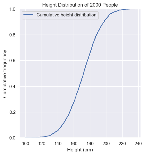
sns.displot(height, kind="ecdf", label="Cumulative height distribution")
plt.xlabel("Height (cm)")
plt.ylabel("Cumulative frequency")
plt.title("Height Distribution of 2000 People")
plt.legend()
plt.show()
Seaborn historgrams
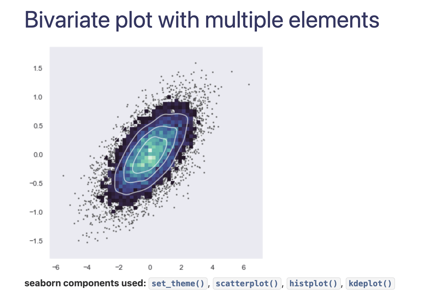
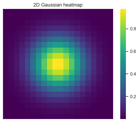
Heatmaps
- Often can be a 2D histogram
- Frequency (or some other feature) is represented with a color scale
Heatmaps
- Can also be used for categorical data
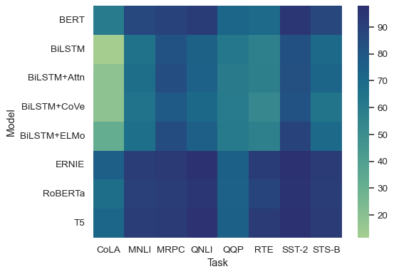
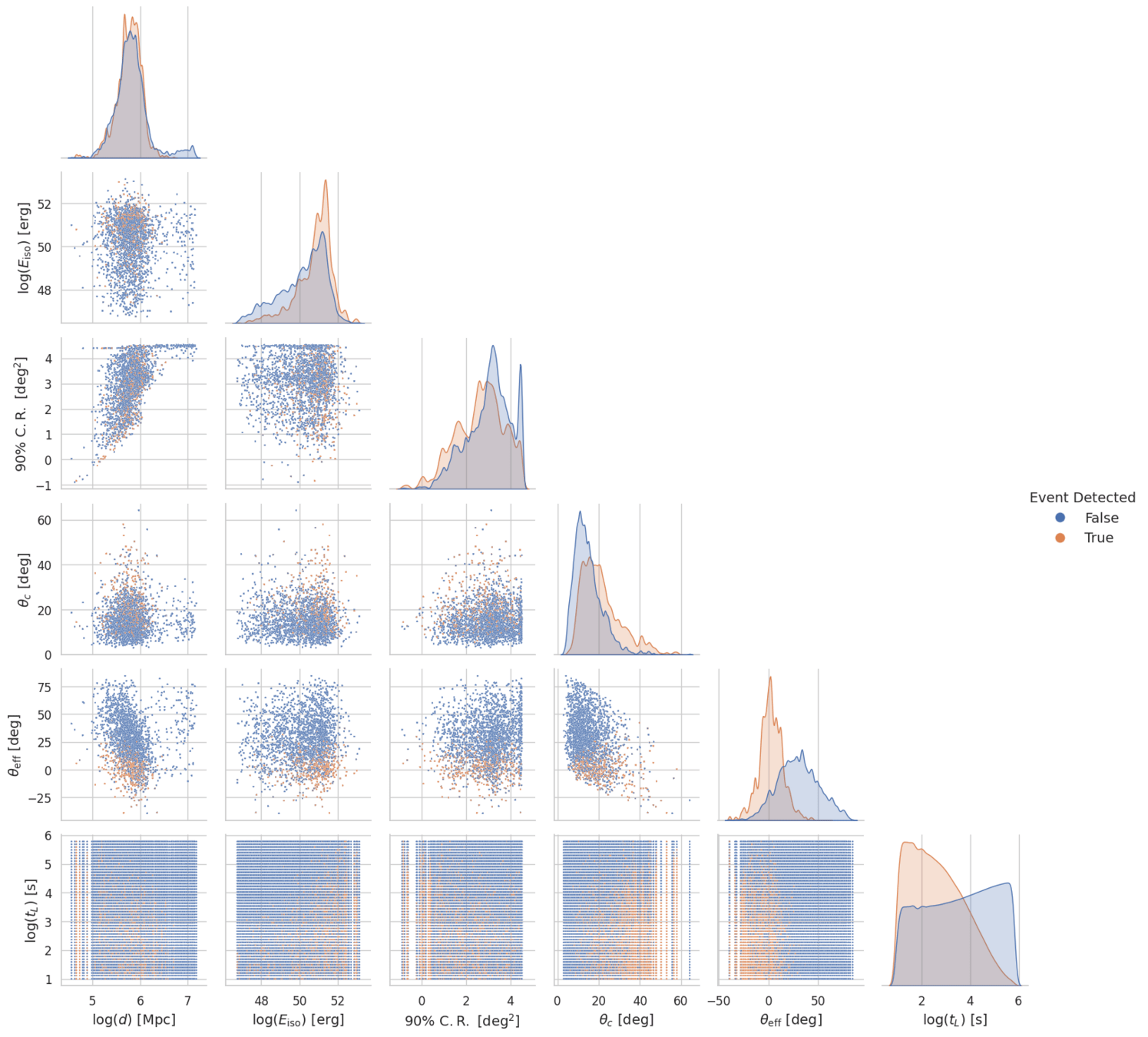
And many more!
Lecture 5
- Recap
- Why visualization
- Matplotlib essentials
- Seaborn quick tour
- Important file formats
Important Data Formats
Plaintext:

.txt
.json
.csv
.xml
.yaml
.toml
Fancier:

.hdf5
.parquet
.lmdb
.SQL
.excel
Plaintext:

.txt
.json
.csv
.xml
.yaml
.toml
Today
Text-based data formats
Plaintext:

.txt
.json
.csv
.xml
.yaml
.toml
Plaintext:

.txt
.json
.csv
.xml
.yaml
.toml
Today
Why so many?
- Different shapes of data havedifferent priorities
- human-readability
- schema strictness
- tabular vs nested
- tooling support
Text-based data formats
Plaintext:

.txt
.json
.csv
.xml
.yaml
.toml
Plaintext:

.txt
.json
.csv
.xml
.yaml
.toml
key-value? Like a dict!
Mental model:
-
.txt → free-form notes/logs
-
.csv → rows & columns (tabular)
-
.json/.xml/.yaml/.toml → nested key–value structures (configs, APIs)
Text files - .txt
-
What: Unstructured plain text; the simplest possible file.
-
Origins: Since the beginning of time
-
Used for:
-
Notes
-
logs
-
docs
-
-
Why use it: Open with any software ever
-
Caveat: No built-in structure
-
you must define your own conventions.
-

Reading text files with Python
with open("lec5.txt", "r") as file:
    data = file.read()

print(data)
- We use this special 'with' format
- When we open a file, we need to remember to close it after reading the data from it
- The 'with' statement automatically closes the file for us once we run all the code underneath it! Thanks 'with'!
Challenge #3
Challenge #3
44 12 96 12 129 120 49 60 38 11 20 478 938 40 102 222 102 23 40 58 40 12 12 12 12 49 60 48 27 37 40 17 172 11 98- Copy the text above and save it to a file called "challenge3.txt"
- Read in the the file and use your Python skills to turn the text into a numpy array of integers
- Calculate the mean and median of the array
CSV
-
What: Comma-Separated Values one row per line
-
Commas to separate columns
-
-
Origins: 1970s
-
Used for: Spreadsheets, databases, etc
-
Why use it: Universal, great for tabular data.
-
Caveats:
-
Schema not embedded
-
Slooooow
-

Reading CSV with Python
import csv

with open("lec5-data/bus.csv", newline="", encoding="utf-8") as f:
    rows = list(csv.DictReader(f))


print(rows)
print(rows[0])

# can also convert to numpy array
data = np.array(rows)
print(data)
date,station,rides
2025-09-05,Central,120
2025-09-05,West,95
2025-09-06,Central,130
2025-09-06,West,105
[{'date': '2025-09-05', 'station': 'Central', 'rides': '120'}
 {'date': '2025-09-05', 'station': 'West', 'rides': '95'}
 {'date': '2025-09-06', 'station': 'Central', 'rides': '130'}
 {'date': '2025-09-06', 'station': 'West', 'rides': '105'}]
JSON
-
What: JavaScript Object Notation
-
Origins: 2000s
-
Used for: Web APIs
-
Most data passed around from websites to you browser is communicated via JSON
-
-
Why use it: Human-readable, things are typed
-
Caveats: No comments allowed! :(

JSON
{
    "users": [
        {
            "name": "Lady Gaga",
            "email": "lady.gaga@mpp.mpg.de",
            "age": 36,
            "signed_in": true
        },
        {
            "name": "David Hasselhoff",
            "email": "david.hasselhoff@tum.de",
            "age": 25,
            "signed_in": false
        },
        {
            "name": "Johann Sebastian Bach",
            "email": "bach@db.de",
            "age": 300,
            "signed_in": true
        }
    ]
}
# json

import json

with open("userinfo.json", "r") as f:
    data = json.load(f)

print(type(data))
print(data["users"][0])
The type is a dictionary!
XML
-
What: eXtensible Markup Language
-
Origins: W3C 1998
-
Used for: document formats (e.g., Office
.docxinside is XML!), config files, RSS, HTML? -
Why use it: uhhhhh....
-
Caveats: Verbose, usually overkill

<?xml version="1.0" encoding="UTF-8"?>
<users>
    <user>
        <name>Lady Gaga</name>
        <email>lady.gaga@mpp.mpg.de</email>
        <age>36</age>
        <signed_in>true</signed_in>
    </user>
    <user>
        <name>David Hasselhoff</name>
        <email>david.hasselhoff@tum.de</email>
        <age>25</age>
        <signed_in>false</signed_in>
    </user>
    <user>
        <name>Johann Sebastian Bach</name>
        <email>bach@db.de</email>
        <age>300</age>
        <signed_in>true</signed_in>
    </user>
</users>
XML
this is the same address book as before
YAML
-
What: YAML Ain’t Markup Language —
-
Origins: ~2001
-
Used for: Python Configs, GitHub Actions, CI/CD
-
Why choose it: Very readable for humans!
-
Caveats: indentation sensitivity

YAML
users:
  - name: Lady Gaga
    email: lady.gaga@mpp.mpg.de
    age: 36
    signed_in: true
  - name: David Hasselhoff
    email: david.hasselhoff@tum.de
    age: 25
    signed_in: false
  - name: Johann Sebastian Bach
    email: bach@db.de
    age: 300
    signed_in: true
# uv add pyyaml
import yaml

with open("lec5-data/userinfo.yaml", "r") as f:
    data = yaml.load(f, Loader=yaml.FullLoader)

print(data)
Also loads into a dictionary!
TOML
-
What: TOML (Tom’s Obvious, Minimal Language)
-
Origins: 2013, by Tom Preston-Werner (a GitHub co-founder!)
-
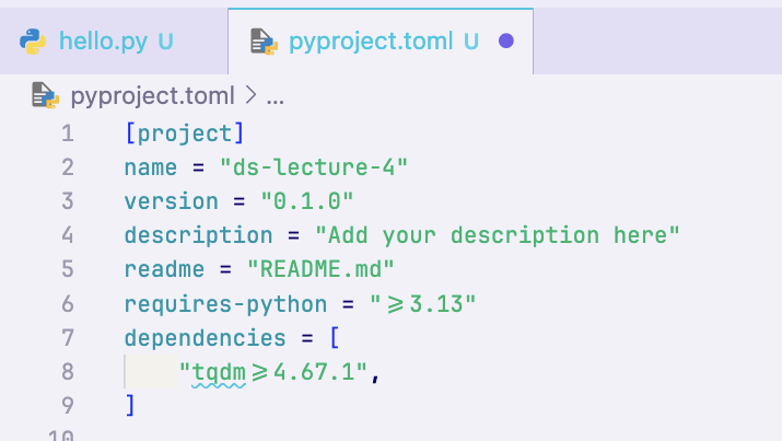
Used for: Python packaging (
pyproject.toml) -
Why choose it: simple grammar, types
-
Caveats: Nested structures are simpler

Reading in TOML files
import tomllib

with open("lec5-data/userinfo.toml", "rb") as f:
    data = tomllib.load(f)
Again, loads into a dictionary!
tomllib included in python since v3.11!
Cheat Sheet
| File Format | When to use |
|---|---|
| CSV | Tabular data, not to much data |
| JSON | Web/API |
| TOML | Human-readable config |
| YAML | Human-readable config |
| XML | Working with super old machine |
| TXT | Notes, logs, etc |
Lecture 5
- Recap
- Why visualization
- Matplotlib essentials
- Seaborn quick tour
- Important file formats
The End
Learning Data Science Lecture 5
By astrojarred
Private


