
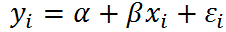
Introduction
Linear Mixed-Effects Model
Generalized Linear Mixed-Effects Model
Hotspots Mapping
Introduction
- We usually assume the samples drawn from targeted population are independent and identically distributed (i.i.d.).
- This assumption does not hold when we have data with multilevel structure:
- clustered and nested data (i.e. individuals within areas)
- longitudinal data (i.e. repeated measurements within individuals)
- non-nested structures (i.e. individuals within areas and belonging to some subgroups such as occupations)
- Samples within each group are dependent, while samples between groups stay independent
- Two sources of variations:
- variations within groups
- variations between groups

- A longitudinal study:
- n = 3
- t = 3
- Complete pooling
- poor performance
- No pooling
- infeasible for large n
- Partial pooling
- An alternative solution: include categorical individual indicators in the traditional linear regression model.
- Why do we still need mixed-effects models?
- Account for both individual- and group-level variations when estimating group-level coefficients.
- Easily model variations among individual-level coefficients, especially when making predictions for new groups.
- Allow us to estimate coefficients for specific groups, even for groups with small n

Fixed and Random Effects
- Random Effects: varying coefficients
- Fixed Effects: varying coefficients that are not themselves modeled
How to decide whether to use fixed-effects or random-effects?
When do mixed-effects models make a difference?
Fixed and Random Effects
Two extreme cases:
- when the group-level variation is very little
- reduce to traditional regression models without group indicators (complete pooling) - when the group-level variation is very large
- reduce to traditional regression models with group indicators (no-pooling)
Little risk to apply a mixed-effects model
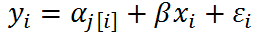
What's the difference between no-pooling models and mixed-effects models only with varying intercepts?
- In no-pooling models, the intercept is obtained by least squares estimates, which equals to the fitted intercepts in models that are run separately by group.
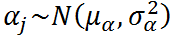
- In mixed-effects models, we assign a probability distribution to the random intercept:

Intraclass Correlation (ICC)
shows the variation between groups
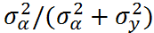
ICC ranges from 0 to 1:
- ICC -> 0: the groups give no information (complete-pooling)
- ICC -> 1: all individuals of a group are identical (no-pooling)
Intraclass Correlation (ICC)
ICC ranges from 0 to 1:
- ICC -> 0: "hard constraint" to
- ICC -> 1: "no constraint" to
- Mixed-effects model: "soft constraint" to


This constraint has different effects on different groups:
- For group with small n, a strong pooling is usually seen, where the value of is close to the mean (towards complete-pooling)
- For group with large n, the pooling will be weak, where the value of is far away from the mean (towards no-pooling)

Linear Mixed-Effects Model
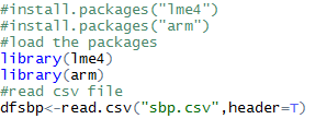
Pull the codes and dataset: https://github.com/benhhu/R-Mixed-Effects-Model
Load the Packages and Data
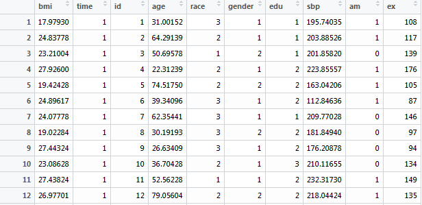
1,000 participants
5 repeated measurements
bmi
time
id
age
race: 1=white, 2=black, 3=others
gender: 1=male, 2=female
edu: 1=<HS, 2=HS, 3=>HS
sbp
am: 1=measured in morning
ex: #days exercised in the past year
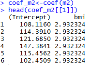
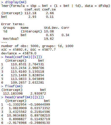
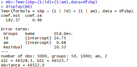
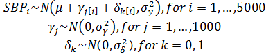
Varying-intercept Model with No Predictors
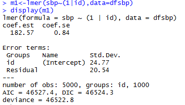
allows intercept to vary by individual
estimated intercept, averaging over the individuals
estimated variations
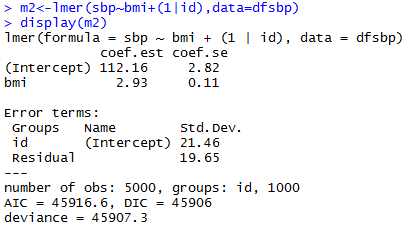
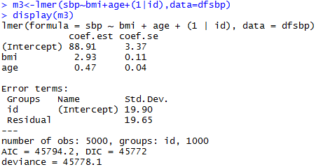
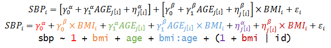
Varying-intercept Model with an individual-level predictor
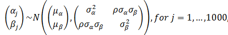
Varying-intercept Model with both individual-level and group-level predictors

Varying Slopes Models
With only an individual-level predictor


Varying Slopes Models
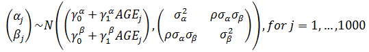
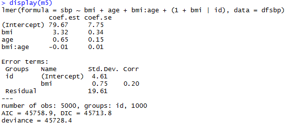
Add a group-level predictor

Non-nested Models
Generalized Linear Mixed-Effects Model
Mixed-Effects Logistic Model
Empty model


Mixed-Effects Logistic Model
Add bmi and race


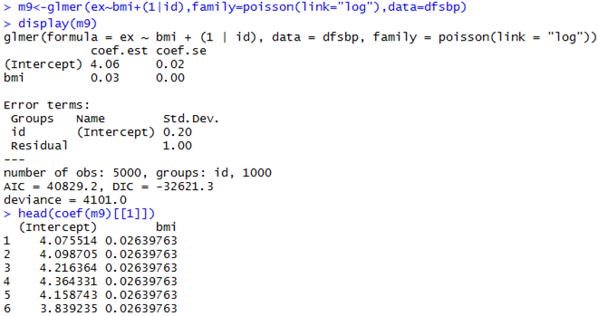
Mixed-Effects Poisson Model

Parameter Estimation Algorithms
- ML: maximum likelihood
- REML: restricted maximum likelihood
- default in lmer() - PQL: pseudo- and penalized quasilikelihood
- Laplace approximations
- default in glmer() - GHQ: Gauss-Hermite quadrature
- McMC: Markov chain Monte Carlo

Bolker BM, Brooks ME, Clark CJ, Geange SW, Poulsen JR, Stevens MHH, et al. 2009. Generalized linear mixed models: A practical guide for ecology and evolution. Trends in ecology & evolution 24:127-135.
Mixed-Effects Model vs. GEE
| Mixed-Effects Model | Marginal Model with GEE | |
|---|---|---|
| Distributional assumptions | Yes | No |
| Population average estimates | Yes | Yes |
| Group-specific estimates | Yes | No |
| Estimate variance components | Yes | No |
| Perform good with small n | Yes | No |
Hotspots Mapping
Introduction to Spatial Data
Data Models
A geographic data model is a structure for organizing geospatial data so that it can be easily stored and retrieved.


Geographic coordinates
Tabular attributes
Spatial Data Models
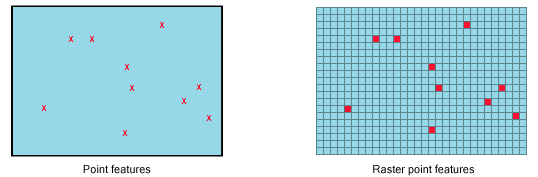
Vector Model
- points, lines, polygons
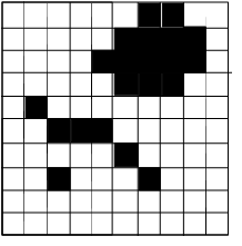
Raster Model
- exhaustive regular or irregular partitioning of space
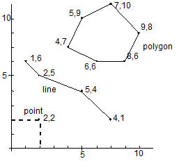
Points
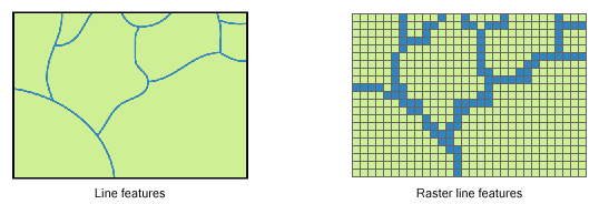
Lines
Shapefiles
.shp - the file that stores the geometry of the feature
.shx - the file that stores the index of the feature geometry
.dbf - the dBASE file that stores the attribute information
.prj - the file that defines the shapefile's projection
.html, .htm, .xml - the files that usually contains metadata
.sbn and .sbx - store additional indices

Coordinate Systems and Projections
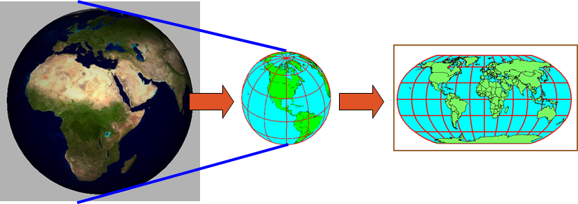
3D sphere
Geographic Coordinate System
2D flat
Projected Coordiate System
Geographic Coordinate Systems
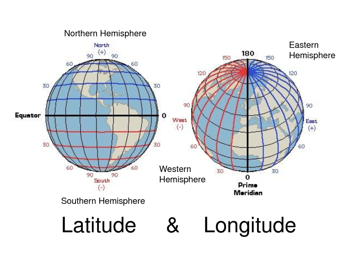
- Longitude and latitude
- Units: Degrees (DMS or DD)
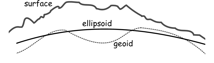
Shape of the Earth
- Surface: The Earth's real surface
- Ellipsoid: Ideal, smooth surface
- Geoid: Bumpy surface, where gravity is equal for all locations
Datum
- Defines the position of the spheroid relative to the center of the earth.
- Global datum:
- uses the earth's center of mass as the origin
- Local datum:
- aligns its spheroid to closely fit the earth's surface in a particular area
- a point on the surface of the spheroid is matched to a particular position on the surface of the earth
- the coordinate system origin of a local datum is not at the center of the earth
Datum
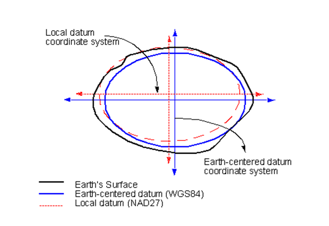
Common Local Datum: North American Datum (NAD)
Common Global Datum: World Geodetic System (WGS)
Projected Coordinate Systems
- A projected coordinate system is defined on a flat, two-dimensional surface
- Unlike a geographic coordinate system, a projected coordinate system has constant lengths, angles, and areas across the two dimensions
- A projected coordinate system is always based on a geographic coordinate system
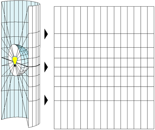
The systematic rendering of a graticule on a flat map surface
Distortion
Converting a sphere to a flat surface results in distortion
-
Shape (conformal) - If a map preserves shape, then feature outlines (like county boundaries) look the same on the map as they do on the earth.
- Lambert Conformal Conic
- UTM -
Area (equal-area) - If a map preserves area, then the size of a feature on a map is the same relative to its size on the earth.
- Alerts Equal Area Conic - Distance (equidistant) - An equidistant map is one that preserves true scale for all straight lines passing through a single, specified point. If a line from a to b on a map is the same distance that it is on the earth, then the map line has true scale. No map has true scale everywhere.
- Direction/Azimuth (azimuthal) – An azimuthal projection is one that preserves direction for all straight lines passing through a single, specified point.
Universal Transverse Mercator Coordinate System
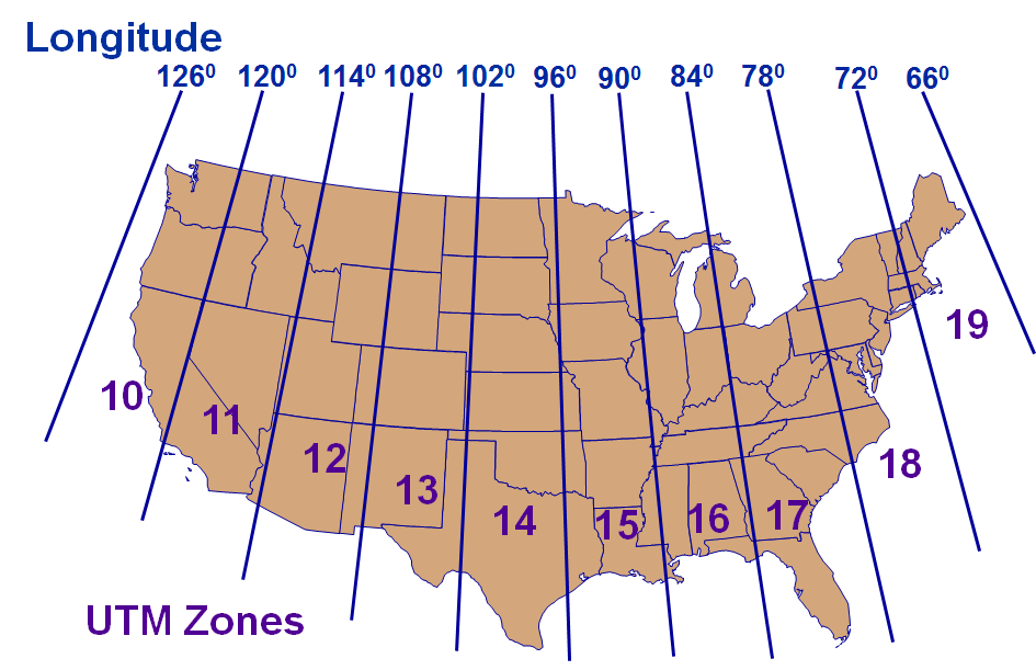
- World divided into 60 six-degree-wide zones
- From 80S to 84N
- Zones numbered 1-60 (N&S), W to E, starting at 180W
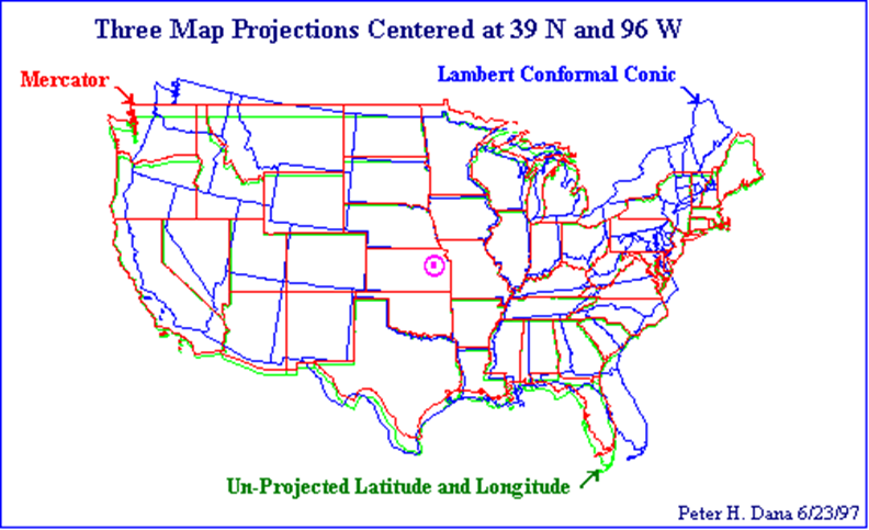
Differences between Projections
Spatial Patterns
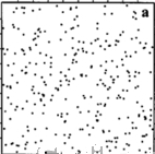
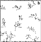
Random
Cluster
Regular
Disease Cluster
- The occurrence of a greater than expected number of cases of a particular disease within a group of people, a geographic area, or a period of time.
- A collection of disease occurrence:
- of sufficient size and concentation to be unlikely to have occurred by chance, or
- related to each other through some social or biological mechanism, or having a common relationship with some other events or circumstance
- Spatial aggregation of disease events may only be a function of the distribution of population
- Disease cluster: residual spatial variation in risk after known influence have been accounted for
Why
- Confirmatory purpose
- verify if a perceived cluster exists
- Exploratory purpose
- searching for spatial patterns
- Identification of clusters can lead to interventions
Methods
- Global clustering:
- evaluate whether clustering exist as a global phenomena throughout the study region, without pinpointing the locaiton of specific cluster
- aggregated data: Moran's I, Geary's C, etc.
- points data: K-nearest neighbour method, etc.
- Local clustering:
- additionally specify the location and can be extended to specify spatial-temporal clusters
Local Clustering
- Focused tests:
- investigate whether there is an increased risk of disease around a predetermined point
- e.g. Superfund site, power plant.
- Lawson Waller score test
- Non-focused tests
- identify the location of all likely clusters in the study region
- LISA, Getis-Ord's local statistics, spatial scan statistics
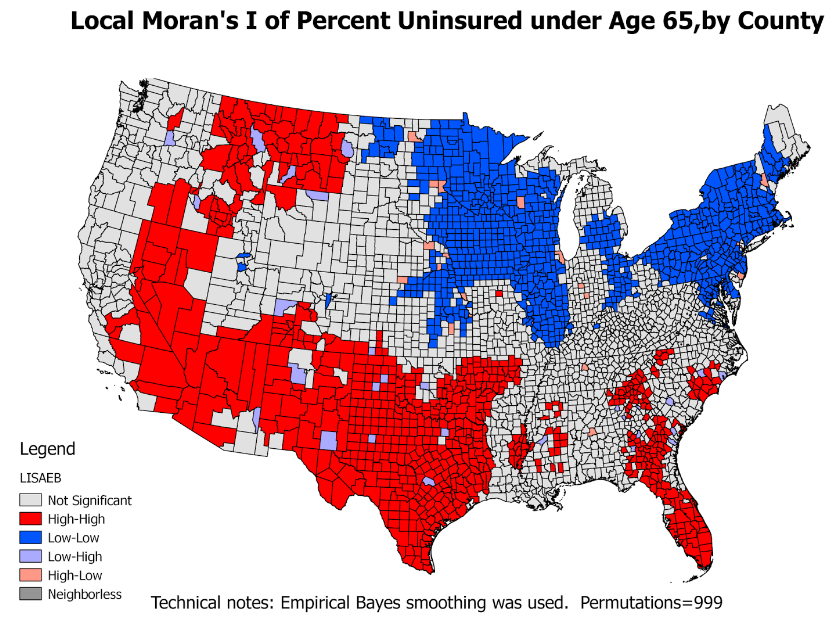
LISA - Local Moran's I
- Local indicators of spatial autocorrelation (LISA)
- show similarity with neighbors and also test its significance
- Divide the study region into 5 categories:
- high-high locations: hot spots
- low-low locations: cold spots
- high-low locations: spatial outliers
- low-high locations: spatial outliers
- Locations with insignificant local autocorrelation
- GeoDa
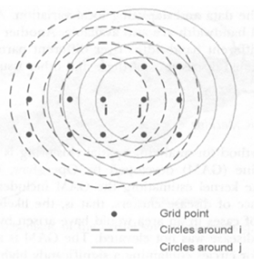
Spatial Scan Statstics
- Search over a given set of spatial regions
- Find those regions which are most likely to be clusters
- Correctly adjust for multiple hypothesis testing
- SatScan
- A circular scanning window is placed at different coordinates with radius that vary from 0 to some set upper limit.
- For each location and size of window
H = elevated risk within window as compared to outside of window
A
Multilevel Approaches - PHC6016
By Hui Hu
Multilevel Approaches - PHC6016
Slides for the Social Epidemiology guest lecture, Fall 2016


