PHC6194 SPATIAL EPIDEMIOLOGY

Ecological Analyses and Mixed-Effect Model
Hui Hu Ph.D.
Department of Epidemiology
College of Public Health and Health Professions & College of Medicine
March 11, 2020
Introduction
Linear Mixed-Effects Model
Generalized Linear Mixed-Effects Model
Project Proposal and Presentation
Introduction
Ecological Studies
- Based on grouped data, with the groups in a spatial context corresponding to geographical areas
- Ecological studies have a long history in many disciplines in addition to epidemiology and public health:
- political science, geography, sociology
- Due to aggregation, ecological studies are susceptible to unique challenges, in particular the potential for ecological bias
- the difference between estimated association based on ecological- and individual-level data
- Ecological data can be used for a variety of purposes:
- mapping: ecological bias is not a big problem (with-in areas variations may be obscured by agggregation)
- cluster detection: small-area anomalies may be washed away when data are aggregated
Ecological Bias
- The fundamental problem with ecological inference is that the process of aggregation reduces information
- this information loss usually prevents identification of parameters of interest in the underlying individual-level model
- If there is no within-area variability in exposures and confounders, then there will be no ecological bias
- therefore, ecological bias occurs due to within-area variability in exposures and confounders
- Distinct consequences of this variability:
- pure specification bias
- confounding
Pure Specification Bias
- Also called model specification bias
- This bias arises because a nonlinear risk model changes its form under aggregation
- This type of bias has nothing to do with confounding
Pure Specification Bias (cont'd)
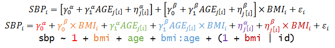
- In an ecological setting, the individual-level data are unavailable, and rather, we observe the aggregate data that correspond to the average outcome and exposure
n_i
Y_{ij}
x_{ij}
# individuals in area i (i=1,2,...,m)
Outcome for individual j in area i
Exposure for individual j in area i
E(Y_{ij}|x_{ij})=\alpha +\beta x_{ij}
\bar y_i = {1 \over n_i} \sum^{n_i}_{j=1}y_{ij}
\bar x_i = {1 \over n_i} \sum^{n_i}_{j=1}x_{ij}
- On aggregation, we have
E(\bar Y_{i}|\bar x_{i})=\alpha +\beta \bar x_{i}
Pure Specification Bias (cont'd)
- Aggregate to sum:
E(Y_{ij}|x_{ij})=\alpha +\beta x_{ij}
E(Y_{i}|x_{ij})=\sum^{n_i}_{j=1} ( \alpha +\beta x_{ij})
- Dividing the left- and right-hand sides by ni
E(Y_{i}|\bar x_{i})=n_i ( \alpha +\beta \bar x_{i})
- When there is no within-area variability in exposure:
x_{ij}=\bar x_i
There is no ecological bias
- The pure specification bias is reduced if areas are smaller, since the heterogeneity of exposures within areas is decreased
Confounding
- It is challenging to characterize the within-area joint distribution of exposures and confounders with only aggregated data
- Two scenarios when we can address the confounding issue with aggregated data
- the exposure and confounders are independent (no interaction between exposure and confounders)
- if we have the confounders that are constant within areas (e.g. county-level policy)
Mixed-Effects Models
- We usually assume the samples drawn from targeted population are independent and identically distributed (i.i.d.).
- This assumption does not hold when we have data with multilevel structure:
- clustered and nested data (i.e. individuals within areas)
- longitudinal data (i.e. repeated measurements within individuals)
- non-nested structures (i.e. individuals within areas and belonging to some subgroups such as occupations)
- Samples within each group are dependent, while samples between groups stay independent
- Two sources of variations:
- variations within groups
- variations between groups

- A longitudinal study:
- n = 3
- t = 3
- Complete pooling
- poor performance
- No pooling
- infeasible for large n
- Partial pooling
- An alternative solution: include categorical individual indicators in the traditional linear regression model.
- Why do we still need mixed-effects models?
- Account for both individual- and group-level variations when estimating group-level coefficients.
- Easily model variations among individual-level coefficients, especially when making predictions for new groups.
- Allow us to estimate coefficients for specific groups, even for groups with small n

Fixed and Random Effects
- Random Effects: varying coefficients
- Fixed Effects: varying coefficients that are not themselves modeled
How to decide whether to use fixed-effects or random-effects?
When do mixed-effects models make a difference?
Fixed and Random Effects
Two extreme cases:
- when the group-level variation is very little
- reduce to traditional regression models without group indicators (complete pooling) - when the group-level variation is very large
- reduce to traditional regression models with group indicators (no-pooling)
Little risk to apply a mixed-effects model
What's the difference between no-pooling models and mixed-effects models only with varying intercepts?
- In no-pooling models, the intercept is obtained by least squares estimates, which equals to the fitted intercepts in models that are run separately by group.
- In mixed-effects models, we assign a probability distribution to the random intercept:

Intraclass Correlation (ICC)
shows the variation between groups
ICC ranges from 0 to 1:
- ICC -> 0: the groups give no information (complete-pooling)
- ICC -> 1: all individuals of a group are identical (no-pooling)
Intraclass Correlation (ICC)
ICC ranges from 0 to 1:
- ICC -> 0: "hard constraint" to
- ICC -> 1: "no constraint" to
- Mixed-effects model: "soft constraint" to


This constraint has different effects on different groups:
- For group with small n, a strong pooling is usually seen, where the value of is close to the mean (towards complete-pooling)
- For group with large n, the pooling will be weak, where the value of is far away from the mean (towards no-pooling)

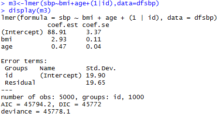
Linear Mixed-Effects Model
git pull
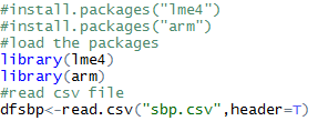
Load the Packages and Data
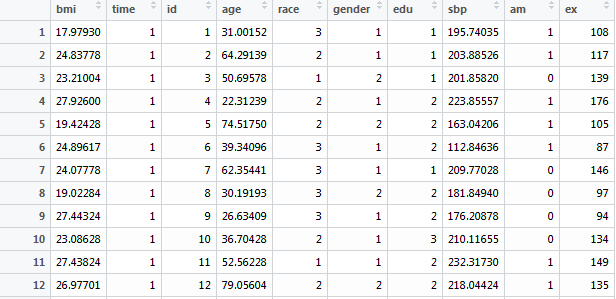
1,000 participants
5 repeated measurements
bmi
time
id
age
race: 1=white, 2=black, 3=others
gender: 1=male, 2=female
edu: 1=<HS, 2=HS, 3=>HS
sbp
am: 1=measured in morning
ex: #days exercised in the past year
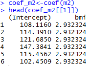
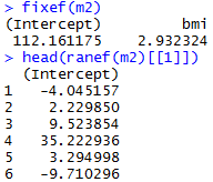
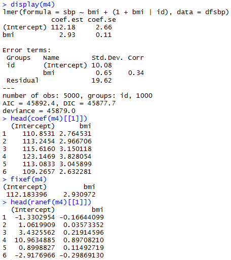
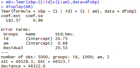
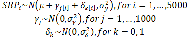
Varying-intercept Model with No Predictors
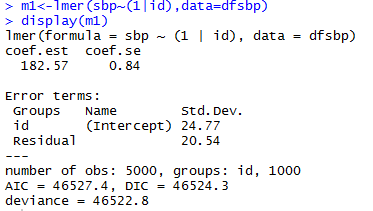
allows intercept to vary by individual
estimated intercept, averaging over the individuals
estimated variations
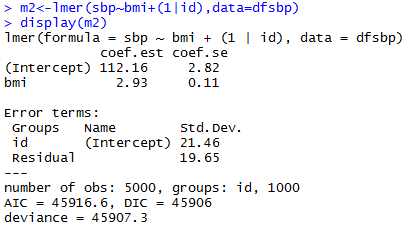
Varying-intercept Model with an individual-level predictor
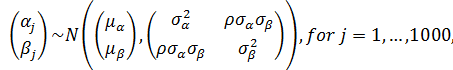
Varying-intercept Model with both individual-level and group-level predictors

Varying Slopes Models
With only an individual-level predictor


Varying Slopes Models
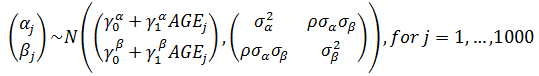
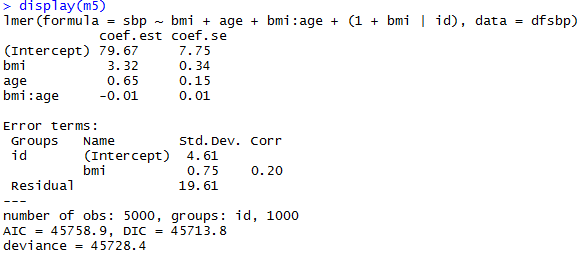
Add a group-level predictor

Non-nested Models
Generalized Linear Mixed-Effects Model
Mixed-Effects Logistic Model
Empty model


Mixed-Effects Logistic Model
Add bmi and race


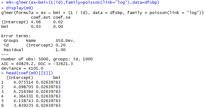
Mixed-Effects Poisson Model

Parameter Estimation Algorithms
- ML: maximum likelihood
- REML: restricted maximum likelihood
- default in lmer() - PQL: pseudo- and penalized quasilikelihood
- Laplace approximations
- default in glmer() - GHQ: Gauss-Hermite quadrature
- McMC: Markov chain Monte Carlo

Bolker BM, Brooks ME, Clark CJ, Geange SW, Poulsen JR, Stevens MHH, et al. 2009. Generalized linear mixed models: A practical guide for ecology and evolution. Trends in ecology & evolution 24:127-135.
Mixed-Effects Model vs. GEE
| Mixed-Effects Model | Marginal Model with GEE | |
|---|---|---|
| Distributional assumptions | Yes | No |
| Population average estimates | Yes | Yes |
| Group-specific estimates | Yes | No |
| Estimate variance components | Yes | No |
| Perform good with small n | Yes | No |
Project Proposal and Presentation
Project Proposal
- Cover Page: Include title and list of team members.
Project description: One-page, and please include the following:
- Specific Aims/Objectives: for those choosing option A, please cite the article you’d like to reproduce and briefly summarize the specific aims/objectives of the article. For those choosing option B, please state your aims/objectives.
- Approach/Research Design
- Timeline
- Literature cited (no page limit); please follow the Vancouver style. - Proposals must use single column and single spacing; Arial or Times New Roman font; font size no smaller than 11 point; tables and figure labels can be in 10 point; 0.5 inch margins.
Project Presentation
- Up to ten (10) slides and no more than 7 minutes of presentation with 3 minutes Q&A
- Please submit the slides on Canvas by 3/16
PHC6194-Spring2021-Lecture9
By Hui Hu
PHC6194-Spring2021-Lecture9
Slides for Lecture 9, Spring 2021, PHC6194 Spatial Epidemiology


