Partial Equilibrium
and Welfare Analysis
Christopher Makler
Stanford University Department of Economics
Econ 50: Lectures 20 and 21
Fundamental Economic Questions
What, as a society, do we produce?
Who gets what?
How do we decide?
If you were an omniscient
"social planner" in charge of everything, how would you
make these decisions?
How do billions of people
coordinate their economic activities?
What does it mean to
"let the market decide"
what to produce?
Responding to Prices
Weeks 4-5: Consumer Theory
Firms face prices and
choose how much to produce
Consumers face prices and
choose how much to buy
Weeks 6-7: Theory of the Firm
Competitive Equilibrium
Consumers and producers are small relative to the market
(like an individual firefly)
and make one decision: how much to buy or sell at the market price.
Equilibrium occurs when
the market price is such that
the total quantity demanded
equals the total quantity supplied
Equilibrium in General
Definition 1: a situation which economic forces are "balanced"
Definition 2: a situation which is
self-replicating: \(x = f(x)\)
Transition dynamics: excess demand and supply
Stability of Equilibria
All forces can be in balance in different ways.
Assumptions of
Perfect Competition
Perfect information
Homogeneous good
Lots of buyers and sellers
Free entry and exit
This Week's Agenda
Today: Baseline Example
Friday: A More Complex Example
- Review: Market demand and supply
- Finding the equilibrium price
- Gross and net consumer surplus
- Producer surplus
- How markets maximize surplus
- Finding market demand with non-identical consumers
- Finding market supply with non-identical firms
- Welfare analysis using Lagrangians
- How markets aggregate preferences
Note: I was initially going to do partial equilibrium today (simple and complex)
and welfare analysis on Friday (simple and complex).
I've changed to doing the simple cases of both topics today;
we'll go into more depth on Friday for those who are interested.
Individual and Market Demand
Individual demand curve, \(d^i(p)\): quantity demanded by consumer \(i\) at each possible price
Market demand sums across all consumers:
\displaystyle D(p) = N_Cd(p)
\displaystyle D(p) = \sum_{i=1}^{N_C}{d^i(p)}
If all of those consumers are identical and demand the same amount \(d(p)\):
There are \(N_C\) consumers, indexed with superscript \(i \in \{1, 2, 3, ..., N_C\}\).
Market demand curve, \(D(p)\): quantity demanded by all consumers at each possible price
Market demand sums across all consumers:
\displaystyle D(p) = \sum_{i=1}^{N_C}{d^i(p)}
Individual and Market Supply
Firm supply curve, \(s^j(p)\): quantity supplied by firm \(j\) at each possible price
Market supply sums across all firms:
\displaystyle S(p) = N_Fs(p)
\displaystyle S(p) = \sum_{j=1}^{N_F}{s^j(p)}
If all of those firms are identical and supply the same amount \(s(p)\):
There are \(N_F\) competitive firms, indexed with superscript \(j \in \{1, 2, 3, ..., N_F\}\).
Market supply curve, \(S(p)\): quantity supplied by all firms at each possible price
Calculating Partial Equilibrium
\displaystyle \sum_{j=1}^{N_F}{q_j^*}
\displaystyle \sum_{i=1}^{N_C}{x_i^*}
Price \(p^*\) is an equilibrium price in a market if:
1. Consumer Optimization: each consumer \(i\) is consuming a quantity \(x_i^*(p^*)\) that solves their utility maximization problem.
2. Firm Optimization: each firm \(j\) is producing a quantity \(q_j^*(p^*)\) that solves their profit maximization problem.
3. Market Clearing: the total quantity demanded by all consumers equals the total quantity supplied by all firms.
p^* = \frac{MU_i(x_i^*)}{\lambda_i}
p^* = MC_j(q_j^*)
=
"Marginal benefit in dollars per unit of good 1"
\underbrace{S(p^*)}
\underbrace{D(p^*)}
\(N_C\) identical consumers, each of whom
has the Cobb-Douglas utility function
\(N_F\) identical firms produce good 1, each of which
has the Cobb-Douglas production function
Week 4: Demand for Good 1
Week 7: Supply of Good 1
d(p_1|p_2,m) = \frac{\alpha m}{p_1}
\displaystyle s(p_1|w,r) = \frac{\overline K p_1}{2w}
u(x_1,x_2) = x_1^\alpha x_2^{1-\alpha}
\displaystyle F(L,K) = \sqrt{LK}
and income \(m\)
and capital fixed in the short run at \(\overline K\)
1. Solve for the equilibrium price and quantity if \(\alpha = \frac{1}{4}, m = 100, N_C = 64, w = 4, \overline K = 2, N_F = 16\)
2. Solve for general formula for the equilibrium price and quantity.
Demand
Supply
pollev.com/chrismakler

Suppose that instead of 16 firms, we had only 9 firms.
Then, we would expect the equilibrium price to _____ and the equilibrium quantity to _____.
(Hint: think about what happens to the market demand and supply curves.)
\displaystyle \sum_{j=1}^{N_F}{s^j(p)}
\displaystyle \sum_{i=1}^{N_C}{d^i(p)}
Important Note: Three Kinds of “=" Signs
1. Mathematical Identity: holds by definition
2. Optimization condition: holds when an agent is optimizing
3. Equilibrium condition: holds when a system is in equilibrium
=
MRS = {MU_1 \over MU_2}
MRS = {p_1 \over p_2}
Is this the “right" price?
If you were an omniscient social planner, could you do "better"
than the price the market "chooses"?
Welfare Analysis:
Consumer and Producer Surplus
The Social Planner's Problem
Suppose you were in charge of the economy.
How would you answer the fundamental economic questions about a particular good?
How to produce it?
Want to produce any given quantity Q
at the lowest possible cost
Who gets to consume it?
How much to produce?
Want to distribute any given quantity Q
to the people who value it the most
Want to choose the quantity Q*
to maximize total surplus
(benefit to consumers minus costs of production)
Example: One Consumer, One Firm
FIRM
CONSUMER
Quasilinear utility function:
u(x_1,x_2) = 10x_1 - {1 \over 2}x_1^2 + x_2
Good 2 is "dollars spent on other goods"
p_2 = 1\text{, 1 util = 1 dollar}
Total benefit (in dollars)
from \(x_1\) units of good 1:
v(x_1) = 10x_1 - {1 \over 2}x_1^2
Total cost function:
c(q) = q + {1 \over 4}q^2
Note: variable costs only
GROSS CONSUMER'S SURPLUS
(total benefit, in dollars)
v(x_1) = 10x_1 - {1 \over 2}x_1^2
Marginal benefit,
in dollars per unit:
v'(x_1) = 10 - x_1
(also MRS, marginal willingness to pay)
TOTAL VARIABLE COST
(dollars)
c(q) = q + {1 \over 4}q^2
Marginal cost,
in dollars per unit:
c'(q) = 1 + {1 \over 2}q
What is the optimal quantity \(Q^*\) to produce and consume?
FIRM
CONSUMER
Total benefit:
v(Q) = 10Q - {1 \over 2}Q^2
Total cost:
c(Q) = Q + {1 \over 4}Q^2
Total welfare:
Marginal welfare from producing another unit:
W(Q) = 10Q - {1 \over 2}Q^2 - [Q + \tfrac{1}{4}Q^2]
W'(Q) = 10 - Q - [1 + \tfrac{1}{2}Q]
=0
10 - Q = 1 + \tfrac{1}{2}Q
Q^* = 6
TOTAL WELFARE
(dollars)
Marginal welfare,
in dollars per unit:
Total benefit to consumers minus total cost to firms
Marginal benefit to consumers minus marginal cost to firms
How do competitive markets
solve this problem?
FIRM
CONSUMER
Maximize net consumer surplus
v(x_1) - e(x_1) = 10x_1 - {1 \over 2}x_1^2 - p_1x_1
Maximize profits
r(q) - c(q) = pq - \left[q + {1 \over 4}q^2\right]
FIRM
CONSUMER
Net benefit from buying \(Q\) units at price \(P\):
TB(Q) - P \times Q
Net benefit from selling \(Q\) units at price \(P\):
P \times Q - TC(Q)
Total welfare:
Marginal welfare from producing another unit:
TB(Q) - P \times Q
P \times Q - TC(Q)
W(Q) =
+
MB(Q) - P
P - MC(Q)
W'(Q) =
+
profit-maximizing
firms set P = MC
utility-maximizing consumers set P = MB
as long as consumers and firms face the same price, markets set MB = MC and maximize total welfare!
"Individual ambition serves the common good." - Adam Smith
If there is a single price in the market that all consumers pay, and all producers receive, and all consumers and producers are “price takers,” then:
Every consumer sets MB = p:
- Everyone’s MB from the last unit bought is the same.
- Cannot increase total benefit by reallocating the good from one consumer to another
Every firm set MC = p:
-
Every firm’s MC from the last unit produced is the same.
-
Cannot reduce total costs by reallocating production from one firm to another
The MB of the last unit consumed by some person
equals the MC of the last unit produced by some firm
Endogenizing the Price
Previously: agents took the price
"as given" (exogenous) - it was determined outside the model
Today: we endogenized
the market price by analyzing the model where it's determined
What happens if not everyone is identical?
Two consumers:
\text{Adam: }u_A(x_1^A,x_2^A) = 8 \ln x_1^A + x_2
\text{Eve: }u_E(x_1^E,x_2^E) = 4 \ln x_1^E + x_2^E
\frac{8}{x_1^A} = p_1
\frac{4}{x_1^E} = p_1
D_1(p) = d_1^A(p_1) + d_1^E(p_1)
d_1^A(p_1) = \frac{8}{p_1}
= \frac{8}{p_1} + \frac{4}{p_1}
= \frac{12}{p_1}
Consumer Optimization: Each consumer sets MRS = price ratio
Market Demand: Sum up individual demands for all people:
MRS = \frac{8}{x_1^A}
MRS = \frac{4}{x_1^E}
d_1^E(p_1) = \frac{4}{p_1}
This leads to the individual demand functions:
pollev.com/chrismakler
p = 2q_S
p = 4q_T
S(p) = s_S(p) + s_T(p)
Two firms: Subway's has \(\overline K = 2\), Togo's has \(\overline K =1\), both pay wage rate \(w = 4\).
s_S(p) = \frac{1}{2}p
s_T(p) = \frac{1}{4}p
=\frac{1}{2}p + \frac{1}{4}p
=\frac{3}{4}p
c_S(q_S) = q_S^2 + 2r
c_T(q_T) = 2q_T^2 + r
f(L) = \sqrt{2\overline KL}
MC = \frac{wq}{\overline K}
c(q) = \frac{wq^2}{2\overline K} + r\overline K
Firm Optimization: Each firm sets P = MC
Market Supply: Sum up individual supply for all firms:
\text{Subway}: f(L) = 2\sqrt{L}
\text{Togo's: }f(L) = \sqrt{2L}
Solving for \(q_S\) and \(q_T\) gives us the firms' individual supply functions:
Let's bring our consumers and firms together!
\text{Adam: }u(x_1,x_2) = 8 \ln x_1 + x_2
\text{Subway}: f(L) = 2\sqrt{L}
\text{Eve: }u(x_1,x_2) = 4 \ln x_1 + x_2
\text{Togo's: }f(L) = \sqrt{2L}
1. Consumer Optimization: each consumer \(i\) is consuming a quantity \(x_i^*(p^*)\) that solves their utility maximization problem.
2. Firm Optimization: each firm \(j\) is producing a quantity \(q_j^*(p^*)\) that solves their profit maximization problem.
3. Market Clearing: the total quantity demanded by all consumers equals the total quantity supplied by all firms.
D(p) = \frac{12}{p}
S(p) =\frac{3}{4}p
\frac{12}{p}
\frac{3}{4}p
=
p^* = 4
x_A^* = 2, x_B^* = 1
q_S^* = 2, q_T^* = 1
Note: if we go back to the individual demand
and supply functions, we get:
Welfare Analysis
FIRMS: SUBWAY AND TOGO'S
CONSUMERS: ADAM AND EVE
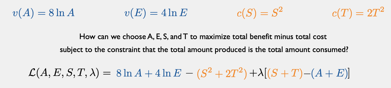
A = number of sandwiches for Adam
v^A(A) = 8 \ln A
v^E(E) = 4 \ln E
S = number of sandwiches produced by Subway
E = number of sandwiches for Eve
T = number of sandwiches produced by Togo's
c^S(S) = S^2
c^T(T) = 2T^2
How can we choose A, E, S, and T to maximize total benefit minus total cost
subject to the constraint that the total amount produced is the total amount consumed?
How Demand
Aggregates Preferences

\Sigma
NOTATION AHEAD
STAY FOCUSED ON
ACTUAL ECONOMICS
Special Case: Cobb-Douglas
u(x_1,x_2,...,x_n) = \alpha_1 \ln x_1 + \alpha_2 \ln x_2 + \cdots + \alpha_n \ln x_n
Suppose each consumer has the utility function
where the \(\alpha\)'s all sum to 1.
x_{k,i}^*(p_1,p_2,...,p_n) = \frac{\alpha_{k,i}\times m_i}{p_k}
We've shown before that if consumer \(i\)'s income is \(m\), their demand for good \(k\) is
quantity demanded of good \(k\) by consumer \(i\)
consumer \(i\)'s preference weighting of good \(k\)
consumer \(i\)'s income
price of good \(k\)
There are 200 people, and they each have \(\alpha = \frac{1}{2}, m = 30\)
u_i(x_1,x_2) = \alpha_i \ln x_1 + (1-\alpha_i) \ln x_2
Suppose there are only two goods, and each consumer has the utility function
x_{1,i}^*(p_1) = \frac{\alpha_{i}\times m_i}{p_1}
So consumer \(i\) will spend fraction \(\alpha_i\) of their income \(m_i\) on good 1:
x_1^*(p_1) = \frac{15}{p_1}
D_1(p_1) = 200 \times \frac{15}{p_1}
Market demand:
= \frac{3000}{p_1}
number of consumers
quantity demanded by each consumer
= \frac{3000}{p_1}
Note: total income is \(200 \times 30 = 6000\), so this means the demand is the same "as if" there were one "representative agent" with \(\alpha = \frac{1}{2}, m = 6000\)
Individual demand:
Now suppose there are two types of consumers:
u_i(x_1,x_2) = \alpha_i \ln x_1 + (1-\alpha_i) \ln x_2
Again there are only two goods, and each consumer has the utility function
x_{1,i}^*(p_1) = \frac{\alpha_{i}\times m_i}{p_1}
x_{1,L}^*(p_1) = \frac{5}{p_1}
x_{1,H}^*(p_1) = \frac{30}{p_1}
D_1(p_1) = \ \ \ \ \ \ \ \ \ \ \ \ \ \ \ \ +
100 low-income consumers who don't like this good: \(\alpha_L = \frac{1}{4}, m_L = 20\)
100 high-income consumers who do like this good:\(\alpha_H = \frac{3}{4}, m_H = 40\)
100\times \frac{30}{p_1}
= \frac{3500}{p_1}
100\times \frac{5}{p_1}
(demand from
low-income)
(demand from
high-income)
\Rightarrow
Market demand:
Individual demand:
Note: total income is \(100 \times 20 + 100 \times 40 = 6000\), so this means the demand is the same "as if" there were one "representative agent" with \(\alpha = \frac{7}{12}, m = 6000\)
Conundrum
In both cases, average income was 30 and average preference parameter \(\alpha\) was \(\frac{1}{2}\).
When everyone was identical, it was "as if"
there was a representative agent with all the money
with preference parameter \(\alpha = \frac{1}{2}\).
When rich people had a higher \(\alpha\), it was "as if"
there was a representative agent with all the money
with preference parameter \(\alpha = \frac{7}{12} > \frac{1}{2}\).
Feel free to tune out the intermediate steps, but hang on to the econ...
How market demand aggregates preferences
x_{k,i}^*(p_1,p_2,p_3,...,p_n) = \frac{\alpha_{k,i} m_i}{p_k}
If consumer \(i\)'s demand for good \(k\) is
then the market demand for good \(k\) is
\displaystyle = \sum_{i=1}^{N_C}\frac{\alpha_{k,i} m_i}{p_k}
\displaystyle = \frac{\alpha_k M}{p_k}
\displaystyle D_k(p_k) = \sum_{i=1}^{N_C}x_{k,i}^*(p_k)
where \(M = \sum m_i\) is the total income of all consumers
and \(\alpha_k\) is an "aggregate preference" parameter.
Conclusion: we can model demand from \(N_C\) consumers with Cobb-Douglas preferences
"as if" they were a single consumer with "average" Cobb-Douglas preferences.
so what is \(\alpha_K\)?
\displaystyle \text{We want to get from }D(p) = \sum_{i=1}^{N_C}\frac{\alpha_{k,i} m_i}{p_k}\text{ to }D(p) = \frac {\alpha_k M}{p_k}
If everyone has the same income (\(m_i = \overline m\) for all \(i\)), then demand simply aggregates preferences:
Let \( \overline m = M/N_C\) be the average income. Then we can rewrite market demand as:
\displaystyle D_k(p_k) = \sum_{i=1}^{N_C}\frac{\alpha_{k,i} m_i}{p_k} \times \frac{M}{N_C \overline m}
\displaystyle = \frac{1}{N_C}\sum_{i=1}^{N_C}\left(\alpha_{k,i} \times \frac{ m_i}{\overline m}\right) \times \frac{M}{p}
\(\alpha_K\)
\displaystyle \alpha_k = \frac{1}{N_C}\sum_{i=1}^{N_C}\alpha_{k,i}
But if there is income inequality, \(\alpha_k\) gives more weight to the prefs of those with higher income.
\(=1\)
Example: consider an economy in which rich consumers like a good more:
100 low-income people with \(\alpha_L = \frac{1}{4}, m_L = 20\),
100 high-income people with \(\alpha_H = \frac{3}{4}, m_H = 40\)
\displaystyle \alpha = \frac{1}{N_C}\sum_{i=1}^{N_C}\left(\alpha_{i} \times \frac{ m_i}{\overline m}\right)
\displaystyle = \frac{1}{200}\left[100 \times \left(\frac{1}{4} \times \frac{20}{30}\right) + 100 \times \left(\frac{3}{4} \times \frac{40}{30}\right)\right]
\displaystyle = \frac{7}{12}
Average income is \(\overline m = 30\), total income is \(M = 6000\)
So, market demand is
\displaystyle D(p) = \alpha \times \frac{M}{p} = \frac{7}{12} \times \frac{6000}{p} = \frac{3500}{p}
closer to \(\alpha_H\) than \(\alpha_L\)
Example, revisited
Source: zillow.com, 5/26/23

Conclusion: Aggregating Preferences
You can model market demand as reflecting the preferences of a single representative agent.
But...know that you're weighting the preferences of richer people more.
Econ 50 | Spring 2023 | Lectures 20 and 21
By Chris Makler
Econ 50 | Spring 2023 | Lectures 20 and 21
Bringing supply and demand together


