pollev.com/chrismakler

Who is the hottest?


Sabrina
Barry
Shawn
You right now
Christopher Makler
Stanford University Department of Economics
Econ 50: Lecture 5
Resource Constraints and Production Possibilities
Today's Agenda
From production functions to the PPF
Getting situated in "Good 1 - Good 2 space"
Resource constraints and the PPF
Deriving the equation of the short-run PPF
The Marginal Rate of Transformation (MRT)
Shifts in technology and the long-run PPF
Good 1 - Good 2 Space
x_1
x_2
Two "Goods" (e.g. fish and coconuts)
A bundle is some quantity of each good
\text{Bundle }X = (x_1,x_2)
x_1 = \text{quantity of good 1 in bundle }X
x_2 = \text{quantity of good 2 in bundle }X
Can plot this in a graph with \(x_1\) on the horizontal axis and \(x_2\) on the vertical axis
A = (4,16)
B = (8,8)
A
B
4
8
12
16
20
4
8
12
16
20
Good 1 - Good 2 Space
x_1
x_2
What tradeoff is represented by moving
from bundle A to bundle B?
\text{Give up }\Delta x_2 =
A
B
4
8
12
16
20
4
8
12
16
20
\text{Gain }\Delta x_1 =
\text{Rate of exchange }=
ANY SLOPE IN
GOOD 1 - GOOD 2 SPACE
IS MEASURED IN
UNITS OF GOOD 2
PER UNIT OF GOOD 1
ANY SLOPE IN
GOOD 1 - GOOD 2 SPACE
IS MEASURED IN
UNITS OF GOOD 2
PER UNIT OF GOOD 1
TW: HORRIBLE STROBE EFFECT!
Multiple Uses of Resources
Labor
Fish
🐟
Coconuts
🥥
[GOOD 1]
⏳
[GOOD 2]
L_1
L_2
\overline L
Resource Constraint
L_1
L_2
L_1 + L_2 = \overline L
\overline L
\overline L
\text{Total labor available }=\overline L
Production Possibilities
\text{Fish }(x_1)
\text{Coconuts }(x_2)
Resource Constraint
L_1
L_2
L_1 + L_2 = \overline L
\overline L
\overline L
\text{Total labor available }=\overline L
\text{(Good 1 - Good 2 space)}
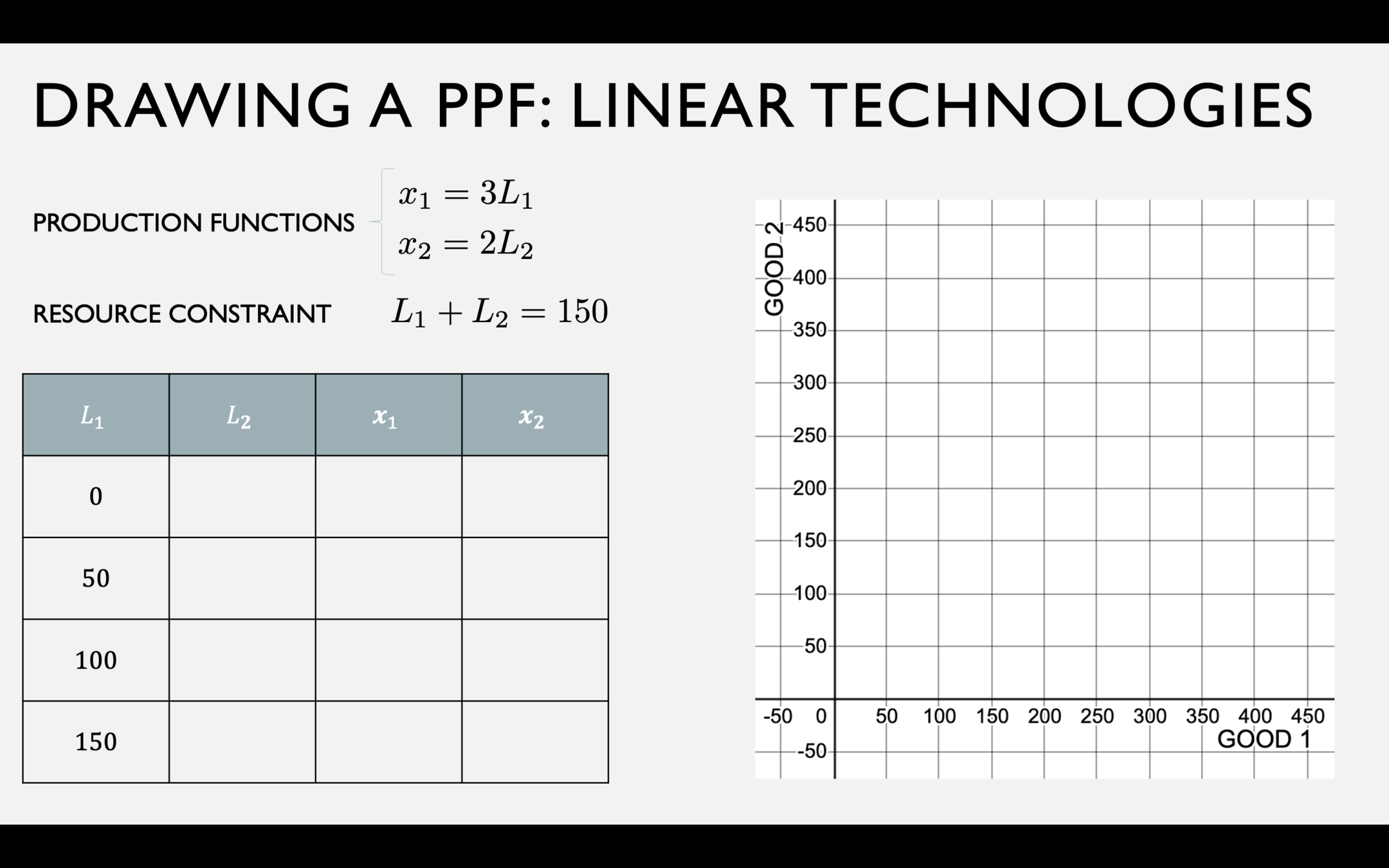
150
100
50
0
0
3 \times 50
150
450
0
2 \times 150
300
200
2 \times 100
300
100
PPF
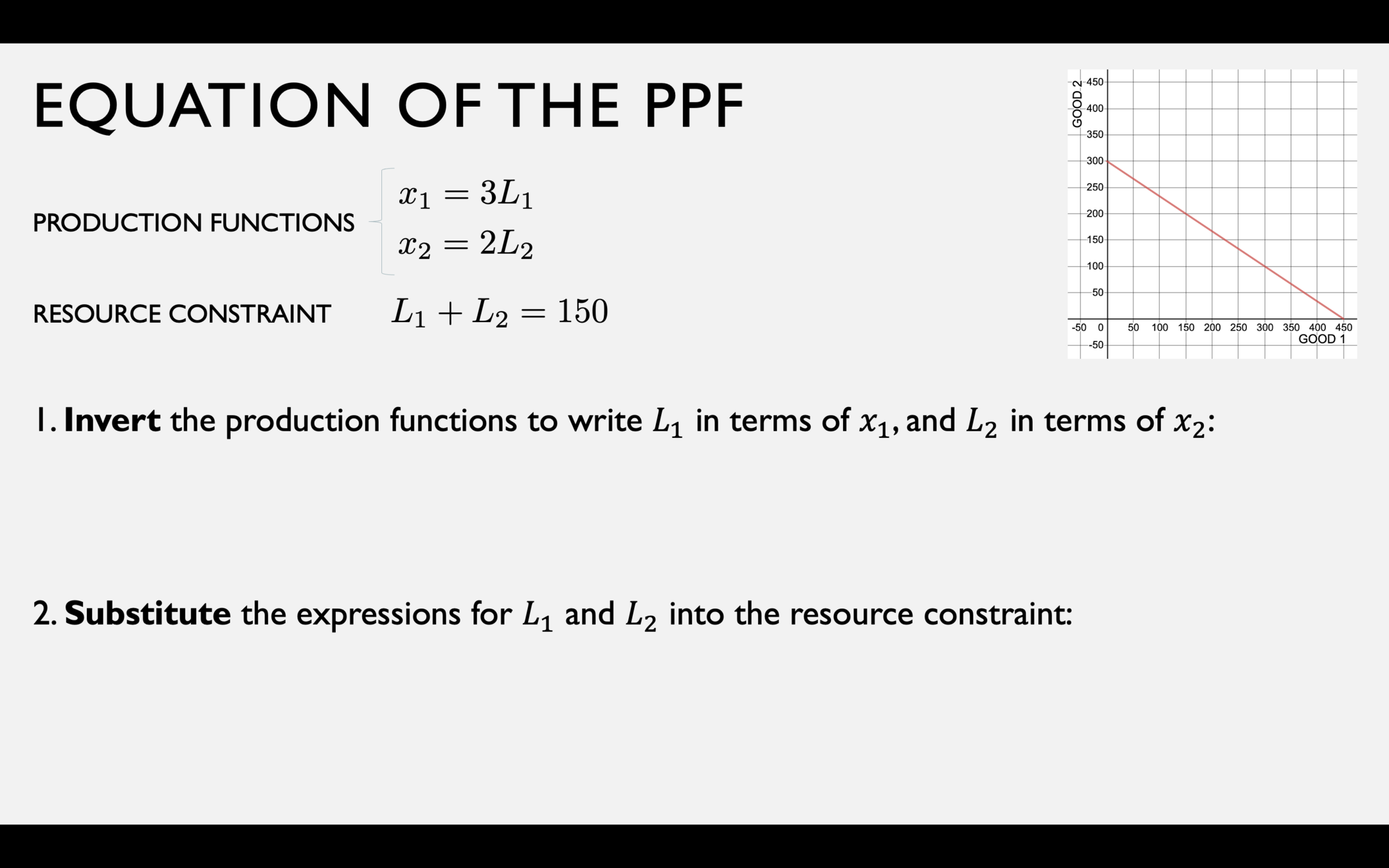
L_1 = {1 \over 3}x_1
L_2 = {1 \over 2}x_2
L_1
+
L_2
= 150
{1 \over 3}x_1
{1 \over 2}x_2
L_1 = {1 \over 3}x_1
L_2 = {1 \over 2}x_2
+
= 150
{1 \over 3}x_1
{1 \over 2}x_2
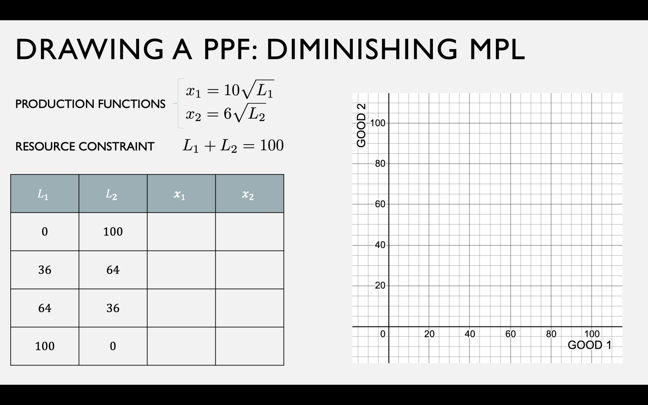

0
10\sqrt{36}
60
100
0
6\sqrt{100}
60
48
6 \sqrt{64}
80
36
PPF
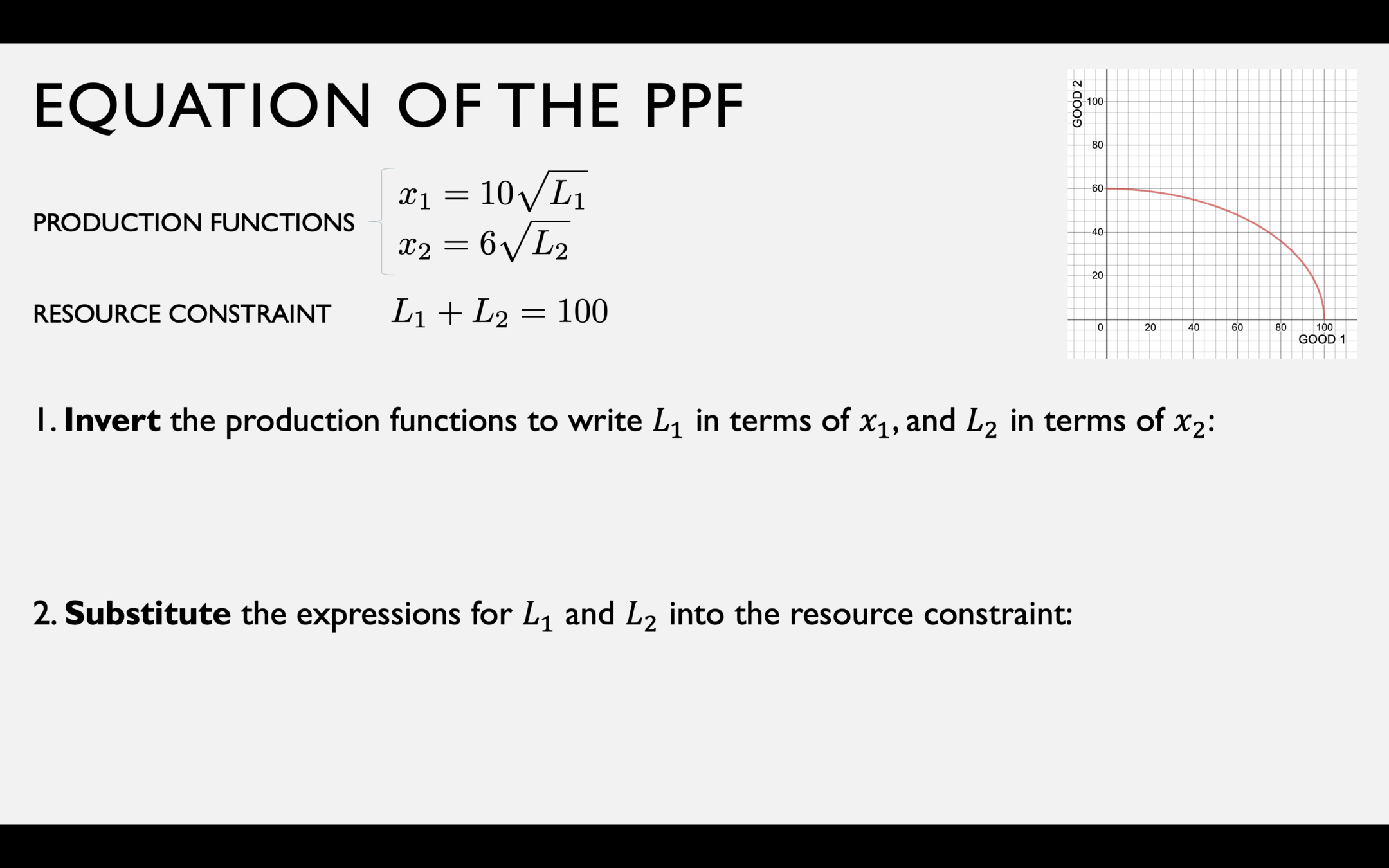
L_1 = {1 \over 100}x_1^2
L_2 = {1 \over 36}x_2^2
L_1
+
L_2
= 100
{1 \over 100}x_1^2
{1 \over 36}x_2^2
L_1 = {1 \over 100}x_1^2
L_2 = {1 \over 36}x_2^2
+
= 100
{1 \over 100}x_1^2
{1 \over 36}x_2^2
Slope of the PPF:
Marginal Rate of Transformation (MRT)
Rate at which one good may be “transformed" into another
...by reallocating resources from one to the other.
Opportunity cost of producing an additional unit of good 1,
in terms of good 2
Note: we will generally treat this as a positive number
(the magnitude of the slope)
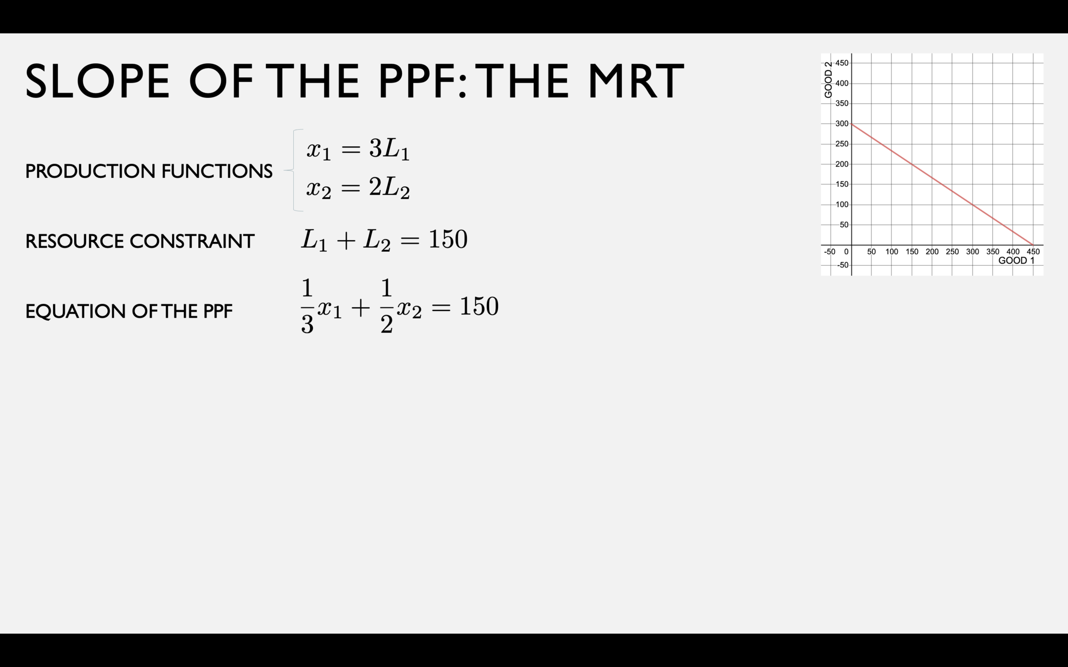
In this simple linear case, we can just solve:
x_2 = 300 - \tfrac{2}{3}x_1
\displaystyle{\Rightarrow MRT = \left|{dx_2 \over dx_1}\right| = {2 \over 3}}
\displaystyle{MRT = \left|{dx_2 \over dx_1}\right| = {2 \over 3}}
It takes \({1 \over 3}\) of an hour (20 minutes)
to make another
unit of good 1
It takes \({1 \over 2}\) of an hour (30 minutes)
to make another
unit of good 2
If you spend 20 more minutes to make another unit of good 1, how much good 2 could you have made in that same 20 minutes?
pollev.com/chrismakler
Suppose Chuck can use labor
to produce fish (good 1)
or coconuts (good 2).
If we plot his PPF in good 1 - good 2 space, what are the units of Chuck's MRT?
Suppose Chuck could initially produce 3 fish (good 1) or 2 coconuts (good 2)
in an hour.
He gets better at fishing, which allows him to produce 4 fish per hour.
What effect will this have on his MRT?
CHECK YOUR UNDERSTANDING
pollev.com/chrismakler
- Suppose we want to produce a lot more of something -- ventilators, masks, toilet paper, hand sanitizer
- Some resources can be reallocated quickly; others are more specialized and can't be quickly repurposed
- How can we "scale up" in the short run and the long run?
- How do short-run tradeoffs compare with long-run tradeoffs?
Shifts in the PPF
f_1(L_1) = {5 \over 4}\sqrt{L_1K_1}
f_2(L_2) = \sqrt{L_2K_2}
Consider an economy with \(\overline L = 100\) units of labor and \(\overline K = 100\) units of capital.
In the short run, \(K_1 = 64\) and \(K_2 = 36\).
In the long run, capital can be reallocated in any combination between goods 1 and 2.
Max in SR
Max in LR
- Up to now: how a short-run PPF can shift due to changing the allocation of capital, holding production functions constant.
- What happens when the technology itself (i.e. the production function) changes?
Improvements in Technology
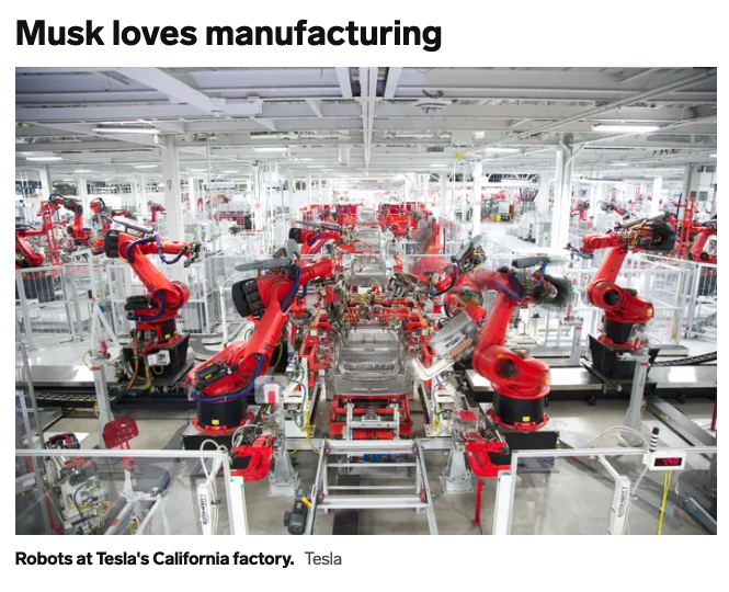
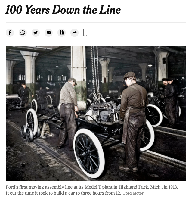
The New York Times, Oct. 29, 2013
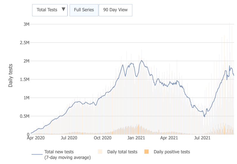
Insider, July 23, 2020
f_1(L_1) = A_1\sqrt{L_1K_1}
f_2(L_2) = A_2\sqrt{L_2K_2}
Consider an economy with \(\overline L = 100\) units of labor and \(\overline K = 100\) units of capital.
In the short run, \(K_1 = 64\) and \(K_2 = 36\).
In the long run, capital can be reallocated in any combination between goods 1 and 2.
Max in SR
Max in LR
- Resource constraints + production functions = production possibilities
- The MRT (slope of PPF) is the opportunity cost of producing good 1
(in terms of good 2). This is affected by the curvature of the production function. - Under the assumptions that capital is fixed in the short run and labor is variable,
- Shifting the allocation of capital affects the short-run PPF
- Changes in technologies affect both the short-run PPF and the long-run PPF
- Section: Introduction to the implicit function theorem (IFT) -- some concrete examples
- Friday: theory of the IFT; using
Key Takeaways
Econ 50 | Lecture 05
By Chris Makler
Econ 50 | Lecture 05
Resource Constraints and Production Possibilities


