pollev.com/chrismakler

Will you need a left-handed desk for exams?
Constrained Optimization When Calculus Works
Christopher Makler
Stanford University Department of Economics
Econ 50: Lecture 10
First Midterm Next Monday!
The homework due Saturday night has several old exam questions as optional exercises.
You don't have to do them all, but you should definitely review the solutions!
Section will be spent reviewing old exam questions.
I will run a review session on Sunday afternoon from 3-5pm, location TBD.
If you have special arrangements, do the paperwork today!
- OAE: upload your form to the link on the web site
- Traveling with a sports team - email me and copy your athletic coordinator
Choice space:
all possible options
Feasible set:
all options available to you
Optimal choice:
Your best choice(s) of the ones available to you
Constrained Optimization

Choice Space
(all colleges plus alternatives)
Feasible Set
(colleges you got into)
Your optimal choice!
Preferences
Preferences describe how the agent ranks all options in the choice space.
For example, we'll assume that you could rank all possible colleges
(and other options for what to do after high school) based upon your preferences.
Preference Ranking
Found a startup
Harvard
Stanford
Play Xbox in parents' basement
Cal
Choice space
Feasible set
Optimal
choice!
Found a startup
Stanford
Cal
Harvard
Play XBox in parents' basement
Optimal choice is the highest-ranking option in the feasible set.
Agenda for Today and Friday
Today: When Calculus Works
Wednesday: When Calculus Doesn't Work
Graphs: PPFs and indifference curves
Words: MRS vs MRT
Math: applying Lagrange
Graphs: PPFs and indifference curves
Words: MRS vs MRT
Math: applying Lagrange
Corner solutions
Kinks
Fish vs. Coconuts
- Can spend your time catching fish (good 1) or collecting coconuts (good 2)
- What is your optimal division of labor between the two?
- Intuitively: if you're optimizing, you couldn't reallocate your time
in a way that would make you better off.
Graphical Analysis:
PPFs and Indifference Curves
The story so far, in two graphs
Production Possibilities Frontier
Resources, Production Functions → Stuff
Indifference Curves
Stuff → Happiness (utility)
Both of these graphs are in the same "Good 1 - Good 2" space
Better to produce
more good 1
and less good 2.
Better to produce
less good 1
and more good 2.
Better to produce
more good 1
and less good 2.
“Gravitational Pull" Towards Optimality
Better to produce
more good 2
and less good 1.
These forces are always true.
In certain circumstances, optimality occurs where MRS = MRT.
Verbal Analysis: MRS, MRT, and the “Gravitational Pull" towards Optimality
Marginal Rate of Transformation (MRT)
- The number of coconuts you need to give up in order to get another fish
- Opportunity cost of fish in terms of coconuts
Marginal Rate of Substitution (MRS)
- The number of coconuts you are willing to give up in order to get another fish
- Willingness to "pay" for fish in terms of coconuts
Both of these are measured in
coconuts per fish
(units of good 2/units of good 1)
Marginal Rate of Transformation (MRT)
- The number of coconuts you need to give up in order to get another fish
- Opportunity cost of fish in terms of coconuts
Marginal Rate of Substitution (MRS)
- The number of coconuts you are willing to give up in order to get another fish
- Willingness to "pay" for fish in terms of coconuts
Opportunity cost of marginal fish produced is less than the number of coconuts
you'd be willing to "pay" for a fish.
Opportunity cost of marginal fish produced is more than the number of coconuts
you'd be willing to "pay" for a fish.
Better to spend less time fishing
and more time making coconuts.
Better to spend more time fishing
and less time collecting coconuts.
Mathematical Analysis:
Lagrange Multipliers
We've just seen that, at least under certain circumstances, the optimal bundle is
"the point along the PPF where MRS = MRT."
CONDITION 1:
CONSTRAINT CONDITION
CONDITION 2:
TANGENCY
CONDITION
This is just an application of the Lagrange method!
Example: Linear PPF, Cobb-Douglas Utility
Chuck has 150 hours of labor, and can produce 3 fish per hour or 2 coconuts per hour.
His preferences may be represented by the utility function \(u(x_1,x_2) = x_1^2x_2\)
To find the equation of his PPF, we invert the production functions and plug them in to the resource constraint:
Production function for fish
Production function for coconuts
Resource constraint
Example 1: Linear PPF, Cobb-Douglas Utility
Chuck has 150 hours of labor, and can produce 3 coconuts per hour or 2 fish per hour.
His preferences may be represented by the utility function \(u(x_1,x_2) = x_1^2x_2\)
OBJECTIVE
FUNCTION
CONSTRAINT
UTILS
HOURS
What are the units?
UTILS
PER
HOUR
FIRST ORDER CONDITIONS
Utility from last hour spent fishing
Utility from last hour spent collecting coconuts
Equation of PPF
Utility from last hour spent fishing
Utility from last hour spent collecting coconuts
Equation of PPF
Equation of PPF
TANGENCY
CONDITION
MRS
MRT
CONSTRAINT
TANGENCY
CONDITION
CONSTRAINT
PLUG INTO
CONSTRAINT
PLUG BACK INTO TANGENCY CONDITION
TANGENCY
CONDITION
CONSTRAINT

TANGENCY
CONDITION
CONSTRAINT
Utility from last hour spent fishing
Utility from last hour spent collecting coconuts
Interpretation of the Lagrange Multplier
At the optimum, we have \(x_1^* = 300\) and \(x_2^* = 100\):
What does this mean?
TANGENCY
CONDITION
CONSTRAINT
PLUG INTO
CONSTRAINT
PLUG BACK INTO TANGENCY CONDITION
How much utility do you get from that bundle?
What is the optimal bundle to produce if you have \(\overline L\) hours of labor available to you?
What is the marginal utility from another hour?
How much utility do you get from that bundle?
What is the optimal bundle to produce if you have \(\overline L\) hours of labor available to you?
What is the marginal utility from another hour?
We found that when \(\overline L = 150\), \(\lambda = 180,000\)

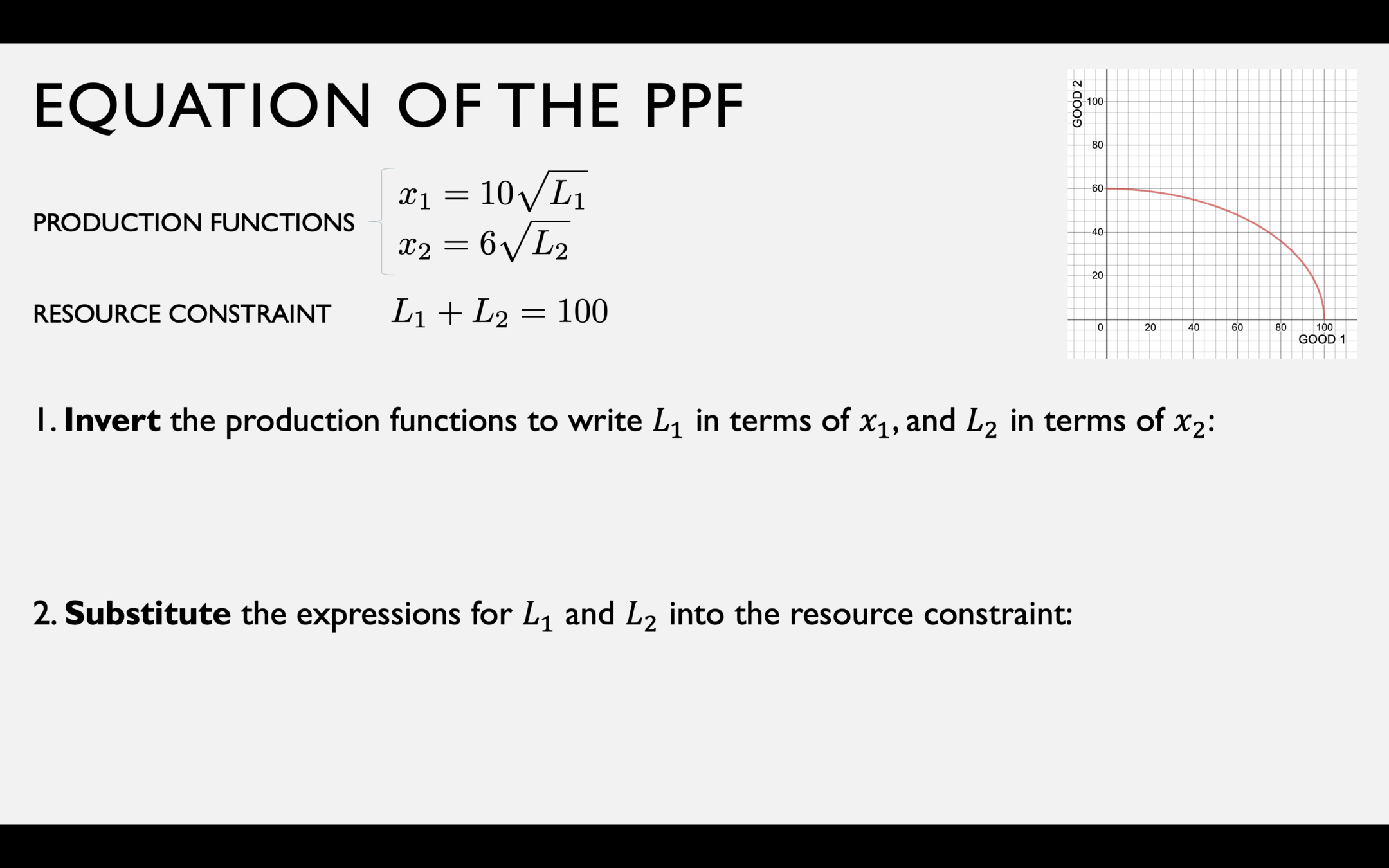
Remember this PPF...let's maximize the Cobb-Douglas utility function \(u(x_1,x_2) = a \ln x_1 + b \ln x_2\) subject to it...
Example 2: Curved PPF, Cobb-Douglas Utility
OBJECTIVE
FUNCTION
CONSTRAINT
First order conditions:
T.C.
CONSTRAINT
(let's square both sides to make substitution easier)
[9/36 = 1/4]
[multiply both sides by \(100a\)]
[factor out \((a + b)\) and divide both sides]
[take the square root]
TANGENCY CONDITION
CONSTRAINT
TANGENCY CONDITION
Remember the setup...
We can rewrite our optimal bundle as
"Spend fraction \(a/(a+b)\) of your labor on good 1, and the rest on good 2."
Tangency Condition
pollev.com/chrismakler

Suppose your preferences may be represented by the utility function
\(u(x_1,x_2) = a \ln x_1 + b \ln x_2\).
What happens to the slope of the line representing the tangency condition if a increases?
Tangency Condition
Summary
- Some decisions are made by balancing your marginal benefits and marginal costs
- If you value something more than its opportunity cost, you should do more of it
- If you value something less than its opportunity cost, you should do less of it
- The Lagrange multiplier method is a mathematical implementation of this:
- The tangency condition finds all value at which MRS = MRT: that is, bundles where your willingness to give up good 2 to get another unit of good 1 (MRS)
is exactly equal to the opportunity cost of another unit of good 1 (MRT). - Adding the constraint condition finds the most affordable such bundle,
given your current resources. - The Lagrange multiplier captures how much more utility you would get from an additional unit of resources.
- The tangency condition finds all value at which MRS = MRT: that is, bundles where your willingness to give up good 2 to get another unit of good 1 (MRS)
- Next time: situations in which your optimal choice is not characterized by this kind of balancing, and Lagrange fails to find the optimum
Econ 50 | Lecture 10
By Chris Makler
Econ 50 | Lecture 10
Constrained Optimization with Calculus
- 894


